How well does the "quick and dirty" standard deviation approximation work?
June 6, 2021
analytics Data science statistics teaching statistics standard deviation
Photo by Chris Liverani on Unsplash.
The standard deviation measures the dispersion of individual samples around a mean value. It is one of the most useful measures in forestry and natural resources because it quantifies the “noise” in a sample of data.
When I was learning statistics in an introductory course, I was shown a formula to approximate the standard deviation. Rather than needing to calculate how far each observation was from the mean value, a key component of the standard deviation calculation, this formula only required knowing the largest and smallest value in the data.
I was intrigued about a calculation that required less work. This meant that an approximation could help with other sampling challenges, typically a result of not having any data about a population of interest. For example, determining the appropriate number of samples to collect at a specified level of confidence requires understanding the variability in a population. Any approximation to the variability would be helpful when performing future analyses.
At the same time, I was skeptical with how well an approximation would capture the true amount of variability in a data set.
This post compares a “quick and dirty” approximation to the standard deviation with its true value. Ten variables from forestry and natural resources are used to make this comparison.
Standard deviation: a primer
When we begin discussing variability in data, we start with the variance. The variance measures the average squared distance of the observations from their mean. To calculate the sample variance \(s^2\), the average of the squared distance is determined:
\[{s^2 = \frac {1}{n-1} {\sum_{i=1}^{n} (x_i- \bar{x})^2}} = \frac {1}{n-1} {(x_1- \bar{x})^2 + (x_2- \bar{x})^2 + ... + (x_n- \bar{x})^2}\] While the variance is used widely in statistics, it is not always a meaningful number to characterize a variable of interest. This is because its units are squared. For a more useful number, instead we’ll take the square root of the variance and report the standard deviation, defined as the average distance of the observations from their mean:
\[{s} = \sqrt{s^2}\]
Two different distributions may have the same mean but different standard deviations. One with a larger standard deviation would have longer “tails” than a distribution with a smaller standard deviation.
The “quick and dirty” approximation to standard deviation
The population mean \(\mu\) and standard deviation \(\sigma\) of a normal distribution help define the empirical rule, a rule that describes the approximate percentages of the range of observations. The empirical rule states that:
- approximately 68% of the observations fall within \(\sigma\) of \(\mu\),
- approximately 95% of the observations fall within \(2\sigma\) of \(\mu\), and
- approximately 99.7% of the observations fall within \(3\sigma\) of \(\mu\).
So, from the empirical rule, we know that nearly all of the data will be found within four standard deviations of the mean (assuming the data are distributed normally). A “quick and dirty” approximation to the standard deviation is \(\sigma \approx \mbox{range}/4\). If you have an estimate of the minimum and maximum values for your variable of interest, you can calculate the range approximate the standard deviation.
Applying the standard deviation approximation
Ten variables from five data sets were compiled to test the approximation assumption with the true standard deviation values. These included:
- The diameter of breast height (
DBH; in) and tons of carbon per acre (Tons) for trees entered in the University of Minnesota’s Carbon Capture Challenge, - The diameter of breast height (
DIA; in), total tree height (HT; ft), and diameter of the tree crown (CROWN_DIAM_WIDE; ft), of cedar elm trees measured in Austin, Texas. - The total amount of forest carbon (
MMT/100; million metric tonnes / 100) in each of 48 US states in 2019, - Measurement of iris flower measurements (cm), including the length of the petal (
Petal.Length) and width of the sepal (Sepal.Width), and - The CO2 concentration (
conc/100) and uptake (uptake) rates of the cold tolerance of a grass species.
The table below shows the approximate and true values for standard deviations:
| Dataset | Variable | SD_true | SD_apxx |
|---|---|---|---|
| carbon | DBH | 13.8 | 14.0 |
| carbon | Tons | 20.0 | 18.5 |
| elm | DIA | 5.1 | 9.5 |
| elm | HT | 9.8 | 13.8 |
| elm | CROWN_DIAM_WIDE | 11.0 | 13.2 |
| state_carbon | MMT/100 | 7.6 | 7.9 |
| iris | Petal.Length | 1.8 | 1.5 |
| iris | Sepal.Width | 0.4 | 0.6 |
| CO2 | conc/100 | 3.0 | 2.3 |
| CO2 | uptake | 10.8 | 9.4 |
The figure below shows the approximate and true values for standard deviations along with a 1:1 line for comparison:
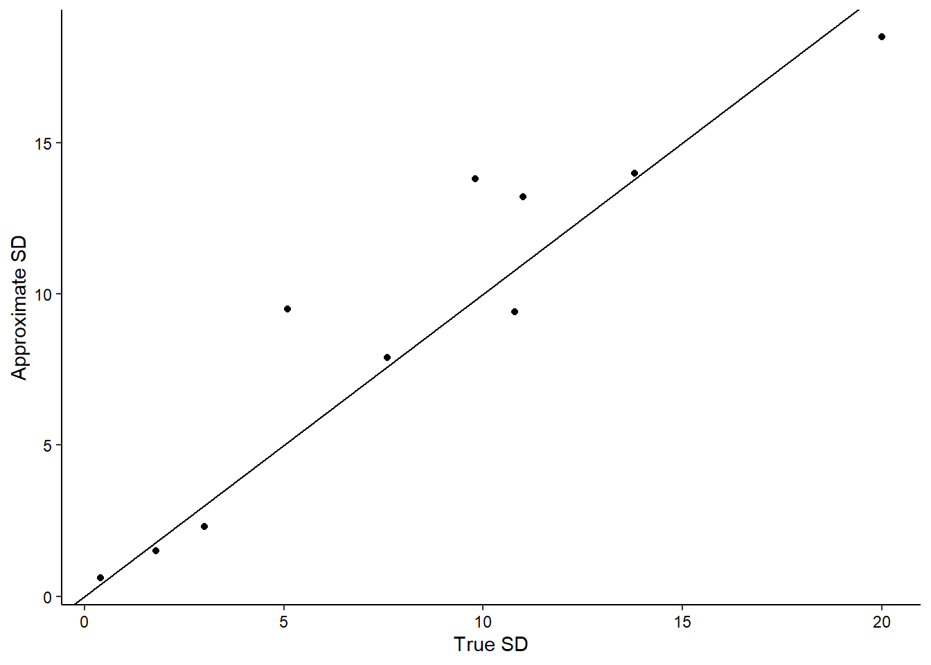
After calculating the differences, the standard deviation approximation was higher than the true value for six of the ten variables. The greatest percent difference for all variables was for the cedar elm diameters (DIA): the true standard deviation was 5.1 inches and the approximation was 9.5 inches. This was likely because of one “outlier” tree that measured 43.0 inches in diameter, yet the next largest tree was 29.0 inches.
Similarly, the HT variable from the cedar elm data set and the Sepal.Width measurement from the iris data set had standard deviation approximations that were more than 38% greater than the true values. These variabilities could have been reduced further by stratifying the data. For example, the cedar elm data could have been separated into their different tree class codes (e.g., open-grown versus dominant trees) and the iris data could have been separated into their different species (e.g., setosa versus versicolor).
Conclusion
The “quick and dirty” standard deviation approximation works well for a sample of data, provided the data are approximately normally distributed. The approximation relies on the range of the data to reflect how noisy the data are. The standard deviation approximation is a quick calculation but should not be used in data where you anticipate extreme values may be present.
–
By Matt Russell. Email Matt with any questions or comments. Sign up for my monthly newsletter for in-depth analysis on data and analytics in the forest products industry.