1. lidR

The lidr package manipulates and visualizes airborne lidar data for forestry applications. It can read and write .las and .laz files and works with point cloud data. An online book has been developed for the package which shows many of its functions and provides tutorials. To install the package:

install.packages("lidR")
library(lidR)

I’ll use an example .las file from NEON of a forest to walk through some functions. The readLAS() function reads in a .las file, and it can be plotted to visualize the forest. The graph output appears in a separate window and enables the user to display, rotate and zoom in on a point cloud:

las <- readLAS("NEONDSSampleLiDARPointCloud.las")
plot(las)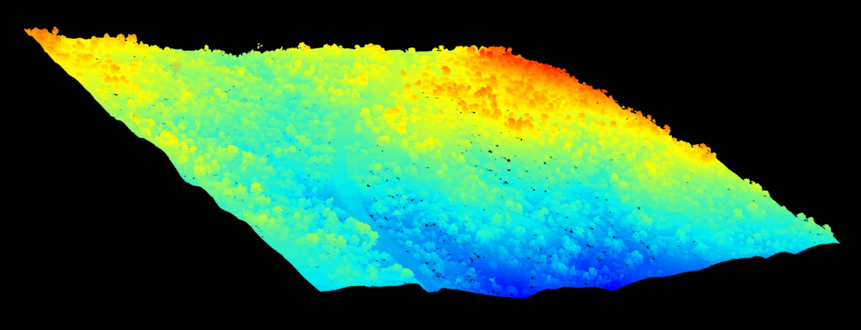

A canopy high model can also be created based on the .las file provided. The package allows for point-to-raster and triangulation approaches to develop the canopy height model. The following code uses the grid_canopy() function to create a canopy height model using an algorithm created by Khosravipour et al.:

thr <- c(0, 2, 5, 10, 15)
edg <- c(0, 1.5)
chm <- grid_canopy(las, 1, pitfree(thr, edg))

plot(chm)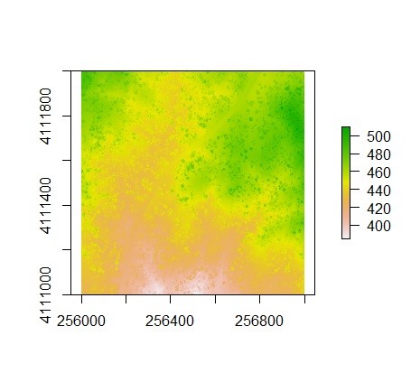

The segment_trees() function allows a user to perform individual tree segmentation, based either on a digital canopy model or the point-cloud:

las <- segment_trees(las, li2012())
col <- random.colors(200)
plot(las, color = "treeID", colorPalette = col)

In addition, the package has several functions for performing wall-to-wall processing across a geographic area of interest. It also works with full waveform lidar data. The package has been installed by users almost 120,000 times.

2. tidyFIA

The tidyFIA package was developed by the forest biometricians at NCX and allows you to download and import data from the USDA Forest Service’s Forest Inventory and Analysis program into your R session. It relies heavily on the tidyverse suite of functions.

Last year I wrote a full tutorial on tidyFIA, and there are a few key functions that are worth highlighting.

To install tidyFIA on your version of R, you can obtain it from GitHub:

remotes::install_github("SilviaTerra/tidyFIA")
library(tidyFIA)

The tidy_fia() function will import any data table from the FIA database using either a state (e.g., states = "MN") or an area of interest. I’ll use the package to import the PLOT table from Minnesota:

mn_data <- tidy_fia(
  states = "MN",
  table_names = c("plot"),
  postgis = FALSE
  )

States with a large volume of data will take some time to load, particularly if you’re using a large table like the TREE table. From here, a number of additional functions are available to query data, plot geospatial distributions of inventory plots, and summarize tree and plot measurements.

The tidyFIA package is a useful one to quickly bring in FIA data into R. It works easily with the tidyverse suite of functions, making it one of my favorites for importing FIA data.

3. rFIA

The rFIA package is another R package that queries and analyzes Forest Inventory and Analysis data. It provides estimates for a variety of forest attributes such as volume, biomass, and carbon stocks. The package has been installed over 15,000 times:

install.packages("rFIA")
library(rFIA)

The getFIA() function downloads FIA data to a specific location in your directory. For example, we can read in all data from Rhode Island, a small state which can illustrate how the functions are used:

ri <- getFIA(states = 'RI', dir = 'C://Users//russellm//Downloads')

The readFIA() function loads the FIA data tables into R from .csv files stored in the local directory you specified:

ri_db <- readFIA('C://Users//russellm//Downloads')

You are able to view each data file contained in your directory, e.g., by typing ri_db$PLOT or ri_db$TREE to view the PLOT and TREE data tables. The tpa() function is one of the most handy functions in the package, providing a basic summary of basal area and trees per acre values for your data:

tpa(ri_db)

## # A tibble: 15 x 8
##     YEAR   TPA   BAA TPA_SE BAA_SE nPlots_TREE nPlots_AREA     N
##    <dbl> <dbl> <dbl>  <dbl>  <dbl>       <int>       <int> <int>
##  1  2005  516.  112.  10.6    3.89          66          67    95
##  2  2006  496.  111.   8.85   3.23          93          95   140
##  3  2007  501.  112.   6.89   3.29         125         126   198
##  4  2008  499.  115.   6.86   3.36         121         122   193
##  5  2009  516.  116.   6.86   3.21         116         118   191
##  6  2010  504.  118.   6.95   3.19         118         119   196
##  7  2011  493.  118.   6.62   3.32         124         127   203
##  8  2012  477.  118.   6.85   3.07         122         125   199
##  9  2013  467.  119.   6.64   3.09         120         123   197
## 10  2014  466.  120.   6.73   3.09         121         123   196
## 11  2015  444.  121.   6.40   3.06         122         124   194
## 12  2016  450.  123.   6.46   2.94         124         125   197
## 13  2017  441.  123.   6.66   3.01         124         125   196
## 14  2018  427.  122.   6.63   3.06         126         127   199
## 15  2019  421.  121.   6.63   3.15         129         130   203

Adding statements such as bySizeClass = TRUE allow you to group the output by diameter class:

tpa(ri_db, bySizeClass = TRUE) 

## # A tibble: 261 x 9
##     YEAR sizeClass    TPA   BAA TPA_SE BAA_SE nPlots_TREE nPlots_AREA     N
##    <dbl>     <dbl>  <dbl> <dbl>  <dbl>  <dbl>       <int>       <int> <int>
##  1  2005         1 231.    4.43  17.1   17.9           41          67    95
##  2  2005         3 108.    8.07  19.1   18.9           30          67    95
##  3  2005         5  58.4  11.3    7.75   7.86          62          67    95
##  4  2005         7  42.7  14.7    5.98   6.06          59          67    95
##  5  2005         9  27.6  14.8    7.50   7.57          57          67    95
##  6  2005        11  19.6  15.1    8.89   9.13          54          67    95
##  7  2005        13  11.4  12.0   12.7   12.5           40          67    95
##  8  2005        15   9.16 12.6   12.8   12.9           39          67    95
##  9  2005        17   3.73  6.45  20.4   20.7           20          67    95
## 10  2005        19   2.24  4.75  28.4   28.3           13          67    95
## # ... with 251 more rows

You can also group the summary statistics by species, a common need in any forest inventory analysis. Incorporating spatial data and producing alternative estimators are also available through a number of functions in rFIA.

4. vegan

The vegan package is a great tool for anyone that regularly needs to produce diversity metrics from forest inventory data. It is branded as a tool for community ecologists and has been installed almost three million times.

install.packages("vegan")

Consider an example data set from the package containing stem counts of trees on one-hectare plots on Barro Colorado Island in the Panama Canal. Data were collected at 50 sites:

library(vegan)
data(BCI)

The specnumber() function defines the number of species for each site and the diversity() function defines the Shannon’s diversity metric for each site:

specnumber(BCI)

##   1   2   3   4   5   6   7   8   9  10  11  12  13  14  15  16  17  18  19  20 
##  93  84  90  94 101  85  82  88  90  94  87  84  93  98  93  93  93  89 109 100 
##  21  22  23  24  25  26  27  28  29  30  31  32  33  34  35  36  37  38  39  40 
##  99  91  99  95 105  91  99  85  86  97  77  88  86  92  83  92  88  82  84  80 
##  41  42  43  44  45  46  47  48  49  50 
## 102  87  86  81  81  86 102  91  91  93

diversity(BCI)

##        1        2        3        4        5        6        7        8 
## 4.018412 3.848471 3.814060 3.976563 3.969940 3.776575 3.836811 3.908381 
##        9       10       11       12       13       14       15       16 
## 3.761331 3.889803 3.859814 3.698414 3.982373 4.017494 3.956635 3.916821 
##       17       18       19       20       21       22       23       24 
## 3.736897 3.944985 4.013094 4.077327 3.969925 3.755413 4.062575 3.979427 
##       25       26       27       28       29       30       31       32 
## 4.074718 3.947749 3.980281 3.693896 3.688721 3.851598 3.724967 3.784873 
##       33       34       35       36       37       38       39       40 
## 3.740392 3.821669 2.641859 3.846109 3.791703 3.516082 3.530494 3.234849 
##       41       42       43       44       45       46       47       48 
## 4.052495 3.966614 3.736254 3.705016 3.609518 3.810489 3.920918 3.913725 
##       49       50 
## 3.778851 3.906616

The Renyi’s measure of diversity is widely used in ecology and can be determined using the renyi() function. The plot() command visualizes the diversity profiles for four randomly selected sites.

k <- sample(nrow(BCI), 4)
R <- renyi(BCI[k,])
plot(R)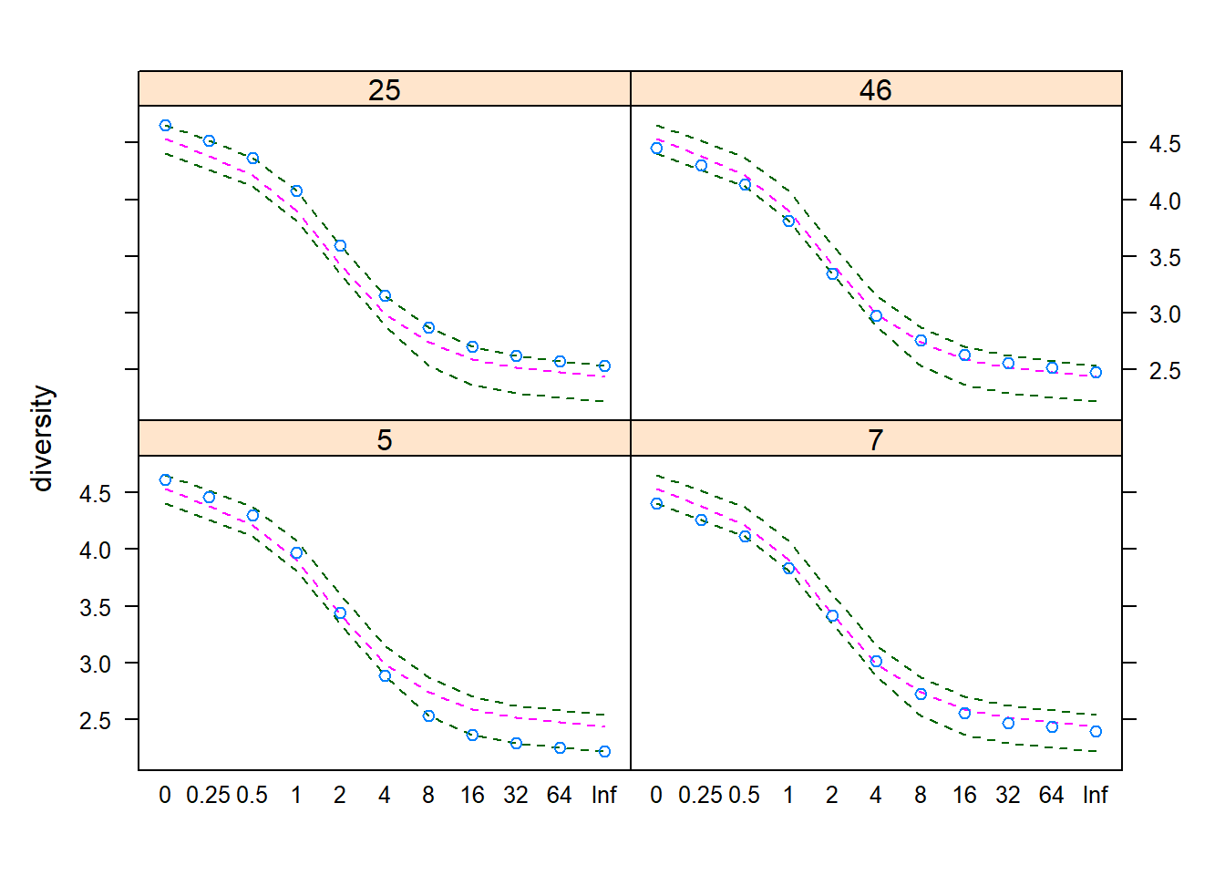

There are a ton more functions that are available in the vegan package, and calculating measures of diversity are just one of a number of tools available. Other functions include ones for partitioning variability in models and performing ordinations and other multivariate analyses.

5. allodb

I recently learned about the allodb package from a colleague. This package was designed to standardize and simplify tree biomass estimation for temperate and boreal forests. The development version can be installed from GitHub:

remotes::install_github("ropensci/allodb")
library(allodb)

The package provides local estimates of aboveground biomass for over 700 species and includes 570 different allometric equations. With all of the interest in generating tree biomass and carbon estimates from trees to stands and landscapes, the package is valuable to efficiently work with tree lists to summarize biomass and carbon attributes.

As an example application, consider four balsam fir and red spruce trees of different diameters growing at the Penobscot Experimental Forest in Maine, USA. The tree data set contains their measurements:

library(tidyverse)

tree <- tribble(
  ~genus, ~species, ~dbh,
  "abies", "balsamea", 10,
  "abies", "balsamea", 20,
  "abies", "balsamea", 30,
  "abies", "balsamea", 40,
  "picea", "rubens", 10,
  "picea", "rubens", 20,
  "picea", "rubens", 30,
  "picea", "rubens", 40
)

The get_biomass() function can be used to determine aboveground biomass (in kg) using species and diameter (in cm):

tree <- tree %>% 
  mutate(agb = get_biomass(dbh = dbh, 
                           genus = genus, 
                           species = species, 
                           coords = c(-68.6, 44.9)))
tree

## # A tibble: 8 x 4
##   genus species    dbh   agb
##   <chr> <chr>    <dbl> <dbl>
## 1 abies balsamea    10  19.8
## 2 abies balsamea    20 121. 
## 3 abies balsamea    30 351. 
## 4 abies balsamea    40 745. 
## 5 picea rubens      10  15.2
## 6 picea rubens      20  91.8
## 7 picea rubens      30 263. 
## 8 picea rubens      40 555.

We can see that balsam fir have slightly greater biomass than red spruce for the same diameter:

ggplot(tree, aes(x = dbh, y = agb, col = species)) +
  geom_point() +
  geom_line()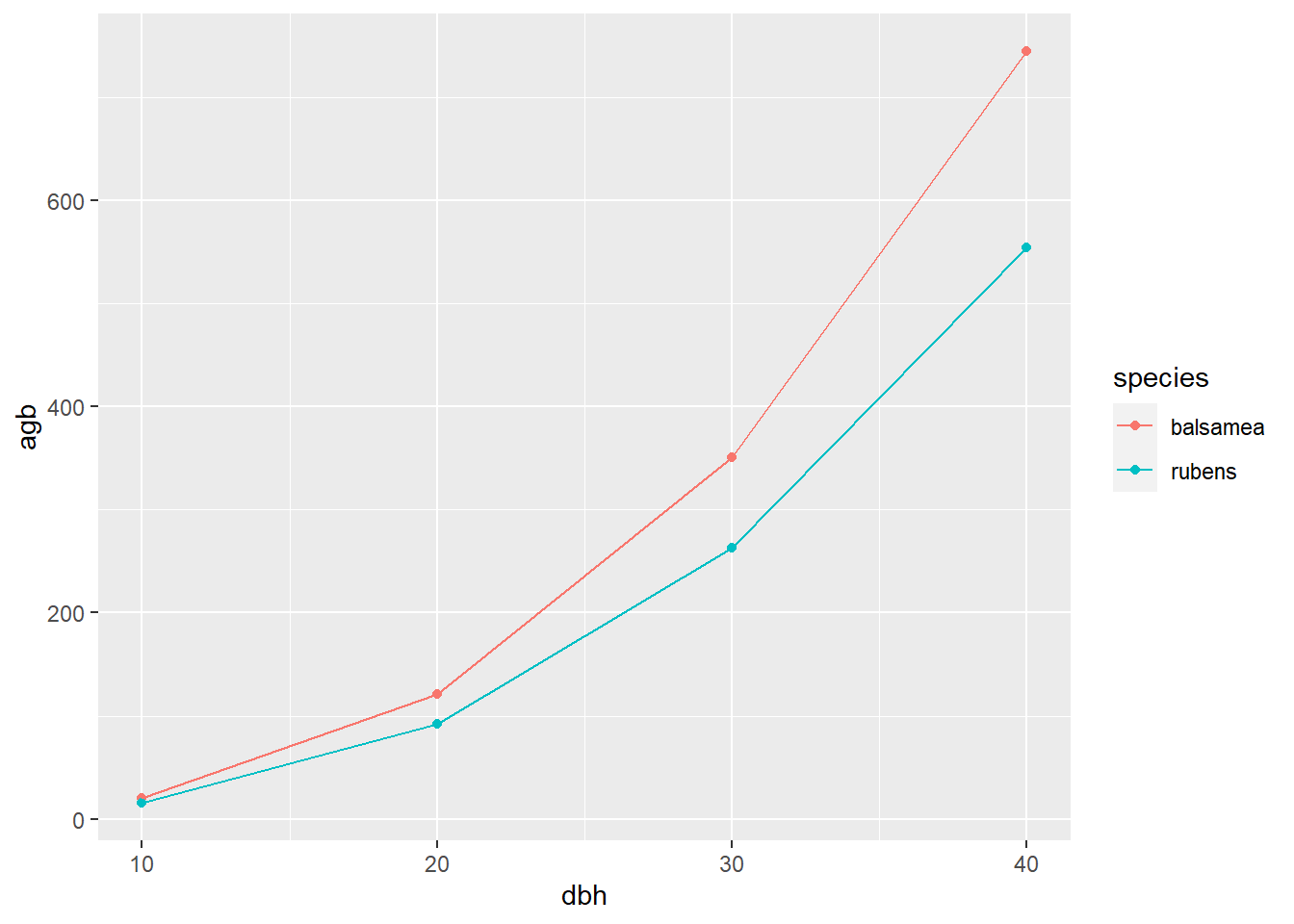

The new_equations() function in allodb allows you to choose a different equation to estimate biomass, or provide your own. You can dig into the package documentation and the supporting article to learn more about the specific equations it uses.

–

Which R package is missing from the list? Email me with your comments and I’d love to hear which forestry packages you use.

–

By Matt Russell. Sign up for my monthly newsletter for in-depth analysis on data and analytics in the forest products industry.