Forget spreading and gathering your R data, try pivoting instead
August 8, 2020
analytics R tidyr pivot_long pivot_wideReshaping data from a wide to a long format, or vice versa, is one of the most common data manipulation tasks that analysts need to do. One of my first posts on this blog was on how to do this in R.
That post highlighted the spread() and gather() functions available from the tidyr package. As it turns out, the gather() and spread() functions are still available to use but are no longer under active development.
Two newer functions available in tidyr are pivot_longer() and pivot_wider(). These functions “lengthen” and “widen” a data set. According to the function documentation, these two functions are designed to be easier to use and can handle more use cases.
To examine how the functions work, say you had an experiment with the number of tree seedlings. These seedlings were initially measured in eight different plots. Five years later the same seedlings were measured again.
The veg data set is formatted long and contains the “pre” (initial) and “post”" (five years later) measurements, along with the number of seedlings per acre:
| PlotID | Period | Seedlings |
|---|---|---|
| 1 | Pre | 1200 |
| 1 | Post | 800 |
| 2 | Pre | 1250 |
| 2 | Post | 950 |
| 3 | Pre | 1350 |
| 3 | Post | 1200 |
| 4 | Pre | 1200 |
| 4 | Post | 650 |
| 5 | Pre | 1100 |
| 5 | Post | 950 |
| 6 | Pre | 1350 |
| 6 | Post | 900 |
| 7 | Pre | 1200 |
| 7 | Post | 650 |
| 8 | Pre | 1240 |
| 8 | Post | 910 |
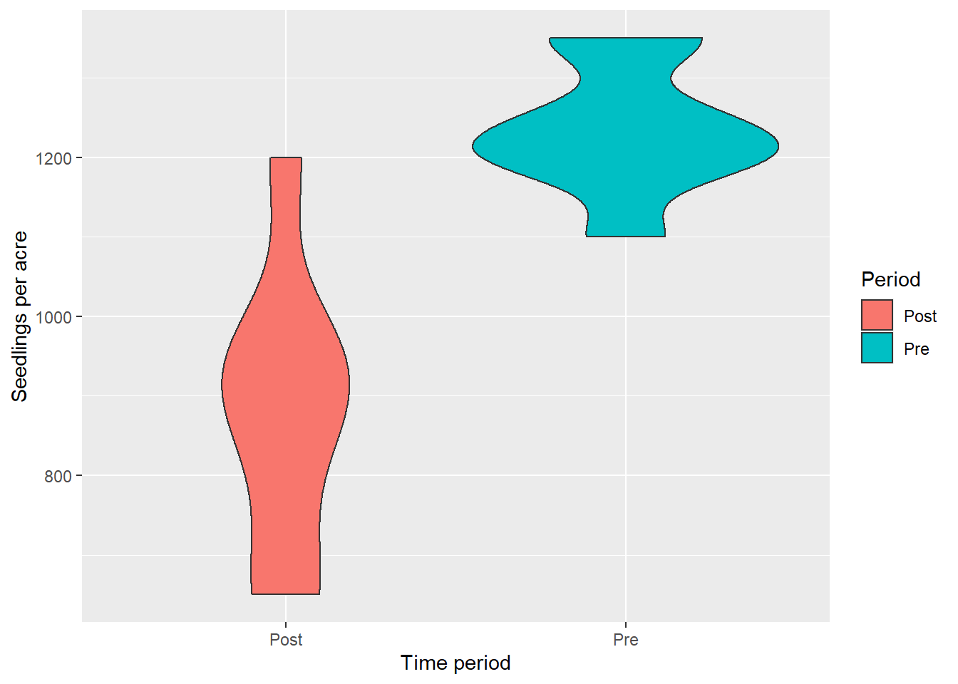
So what happened during the five years? The number of tree seedlings generally decreased. Trees grew larger into the sapling class and many seedlings suffered mortality. Here is a violin plot that shows the trend:
Now, how to visualize the change in tree seedlings between the two measurements? We can convert the veg data to a wide format using the pivot_wider() function from the tidyr package. The result will turn the 16 rows of data into eight rows of data. In this new data set called veg_wide, seedlings will be stored in two columns: the pre and post measurements:
veg_wide <- veg %>%
  pivot_wider(names_from = Period, values_from = Seedlings)
In the names_from argument, you state which column(s) you want to provide in the new output column(s). In our example we create two new columns called Pre and Post that correspond to each of the seedling measurements. In the values_from statement, you state which column(s) to input the cell values into. In our example, are can compare the Pre and Post measurements now that they’re side-by-side:
| PlotID | Pre | Post |
|---|---|---|
| 1 | 1200 | 800 |
| 2 | 1250 | 950 |
| 3 | 1350 | 1200 |
| 4 | 1200 | 650 |
| 5 | 1100 | 950 |
| 6 | 1350 | 900 |
| 7 | 1200 | 650 |
| 8 | 1240 | 910 |
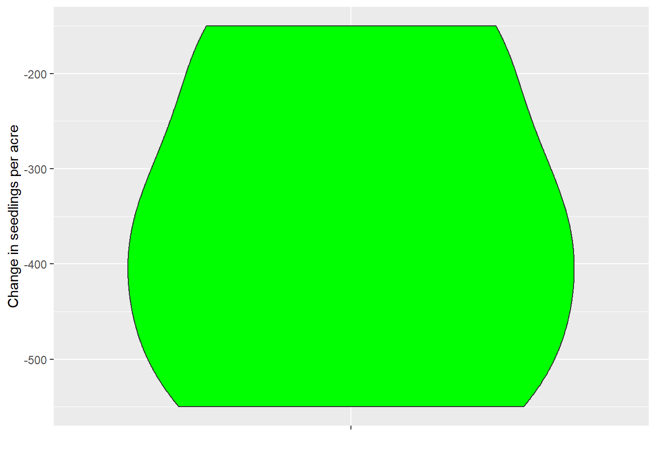
Now we can easily calculate a new variable that quantifies the change in the number of seedlings, called delta_Seedlings. We’ll use the mutate() function:
veg_wide <- veg_wide %>%
  mutate(delta_Seedlings = Post - Pre)
Now we can visualize the primary variable we’re interested in:
The data are now presented in a wide format. Now, we can the pivot_longer() function to make this in a new data frame called veg_long.
veg_long <- veg_wide %>%
  pivot_longer(-PlotID, names_to = "Period", values_to = "Seedlings") %>%
  filter(Period != "delta_Seedlings")
The - operator in the first argument indicates which column(s) you want to pivot (i.e., PlotID). The names_to argument names the new column based on the “wide” column names. We will name this new column Period which will collapse the Pre and Post variables. The values_to argument provides the name of the column to create that was stored in each of the cell values (i.e., the seedling measurements).
Note that the veg_long data set pivots all of the variables in a data set—in our example we suppressed the output of the delta_Seedlings variable using the filter() function from the dplyr package.
Here is how that data set looks:
| PlotID | Period | Seedlings |
|---|---|---|
| 1 | Pre | 1200 |
| 1 | Post | 800 |
| 2 | Pre | 1250 |
| 2 | Post | 950 |
| 3 | Pre | 1350 |
| 3 | Post | 1200 |
| 4 | Pre | 1200 |
| 4 | Post | 650 |
| 5 | Pre | 1100 |
| 5 | Post | 950 |
| 6 | Pre | 1350 |
| 6 | Post | 900 |
| 7 | Pre | 1200 |
| 7 | Post | 650 |
| 8 | Pre | 1240 |
| 8 | Post | 910 |
Look familiar? The veg_long and original veg data sets are identical. Try out the pivot_wider() and pivot_longer() functions the next time you’re reshaping data. They are two of many functions in R for organizing tidy data.
–
By Matt Russell. Sign up for my monthly newsletter for in-depth analysis on data and analytics in the forest products industry.