Carbon is perhaps the most important attribute in trees today. Forests in the United States sequester about 11% of the total CO2 emissions every year, making them an important tool to combat future global changes. Having accurate models that represent how much carbon is stored in trees is essential for understanding their carbon sequestration potential and are widely used in forest carbon accounting tools.
Most equations that predict the amount carbon in a tree start with first predicting its biomass. Approximately half of wood biomass is carbon, which is useful to understand the carbon content in trees of different sizes and species. Weighing the biomass in trees is difficult, but it’s not as difficult as calculating the amount of carbon in a tree.
Biomass equations
Biomass equations for trees are numerous and are developed at local, regional, or national scales. Most biomass equations are relatively simplistic, relying on tree measurements such as diameter and tree species. These simple variables are useful and allow flexibility in applying the equations to a large number of trees. Other variables such as tree height and site conditions will likely increase the accuracy of tree biomass predictions, but come at a cost requiring more detailed information.
One example of biomass equations developed for application in North American forests are those presented in Jenkins et al. 20041. This analysis compiled over 2,600 biomass equations from nearly 200 studies to develop a new set of biomass equations based on tree diameter and species.
We can use R code to write a function named total_AGB that estimates the total aboveground biomass in trees, measured in kg. The equations are based on species group (SPGRP) and a tree’s diameter at breast height, measured in cm (DBH). The values B1 and B2 are parameter estimates that differ by species group:
total_AGB<-function(SPGRP,DBH){
  # First list the parameter estimates for each species group:
if(SPGRP=='Aspen')
  {B1=-2.2094; B2=2.3867}
if(SPGRP=='Cedar/larch')
  {B1=-2.0336; B2=2.2592}
if(SPGRP=='Maple/oak/hickory/beech')
  {B1=-2.0127; B2=2.4342}
if(SPGRP=='Mixed hardwood')
  {B1=-2.48; B2=2.4835}
if(SPGRP=='Pine')
  {B1=-2.5356; B2=2.4349}
if(SPGRP=='Soft maple/birch')
  {B1=-1.9123; B2=2.3651}
if(SPGRP=='Spruce')
  {B1=-2.0773; B2=2.3323}
if(SPGRP=='True fir/hemlock')
  {B1=-2.5384; B2=2.4814}
  # Then calculate total aboveground biomass of each tree (AGB):
  AGB=exp(B1+B2*log(DBH))
    return(AGB=AGB)}
We can graph the biomass functions to see the differences in aboveground biomass for the different species:
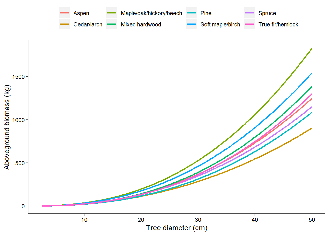
Using these equations, for a given tree diameter, trees in the maple/oak/hickory/beech species group will have the greatest biomass and cedar/larch trees with have the lowest biomass.
Applying the biomass equations to estimate carbon
Consider an example of 10 trees where we’ve measured the species group and tree diameters. We might be interested in estimating the total amount of biomass and carbon in these trees:
| DBH | SPGRP |
|---|---|
| 10 | Pine |
| 14 | Spruce |
| 20 | Maple/oak/hickory/beech |
| 20 | Cedar/larch |
| 25 | True fir/hemlock |
| 30 | Soft maple/birch |
| 33 | Pine |
| 37 | True fir/hemlock |
| 39 | Spruce |
| 45 | Soft maple/birch |
Now, we can apply the total_AGB function to estimate total aboveground biomass and add it as a column in our tree data set:
tree$Biomass<-round(mapply(total_AGB,DBH=tree$DBH,SPGRP=tree$SPGRP),1)Assuming that 50% of wood biomass is carbon, we can also calculate how much carbon is stored in the aboveground portion of the tree, measured in kilograms:
tree$Carbon<-round(tree$Biomass/2,1)Our tree data set now contains estimates of tree biomass and carbon. For example, a maple tree with a DBH of 20 cm has almost twice the amount of carbon compared to the same diameter tree that is a cedar:
| DBH | SPGRP | Biomass | Carbon |
|---|---|---|---|
| 10 | Pine | 21.6 | 10.8 |
| 14 | Spruce | 59.0 | 29.5 |
| 20 | Maple/oak/hickory/beech | 196.3 | 98.2 |
| 20 | Cedar/larch | 113.8 | 56.9 |
| 25 | True fir/hemlock | 232.5 | 116.2 |
| 30 | Soft maple/birch | 460.3 | 230.2 |
| 33 | Pine | 394.7 | 197.3 |
| 37 | True fir/hemlock | 615.1 | 307.6 |
| 39 | Spruce | 643.7 | 321.9 |
| 45 | Soft maple/birch | 1200.9 | 600.5 |
The tree with the greatest amount of carbon, a 45-cm soft maple/birch, contains 600 kg of carbon. Using the Environmental Protection Agency’s Greenhouse Gas Equivalency Calculator, this tree is equivalent to 248 gallons of gasoline consumed or almost 300,000 charges of a smartphone.
Conclusion
Calculating the amount of carbon in trees is an essential analytical tool in forest management. The example presented above is just one application of using existing equations to determine the biomass and carbon content in trees. Linking the amount of carbon stored in trees with a relatable examples such as determining its equivalent in greenhouse gas emissions, helps to educate the public about the role of trees in sequestering carbon.
By Matt Russell. Leave a comment below or email Matt with any questions or comments.
Jenkins, J.C., Chojnacky, D.C., Heath, L.S., Birdsey, R.A., 2004. A comprehensive database of diameter-based regressions for North American tree species. Gen. Tech. Rep. NE-319.↩