Mixed models in R: a primer
October 27, 2020
analytics Data science regression statistics mixed models RMyself and a team of coauthors recently submitted a manuscript that analyzed forest composition data from a silvicultural study. Here is a comment from a peer reviewer that reviewed the work:
“I would like the authors to justify not using mixed models or to change their analyses for mixed models.”
The comment urged us to reevaluate the analysis of the data. Ultimately we redid the analysis using a mixed model framework, instead of using the traditional analysis of variance approach taught in many introductory statistics classes. While the primary results of our study did not change, how we thought about and presented the analysis mattered much more.
Why mixed models?
Mixed models have emerged as one of the go-to regression techniques in forestry applications, largely because forestry data are often nested. This is for several reasons including:
Forestry data are often spatially and temporally correlated. Foresters collect information on plots that are close to one another in space. Permanent sample plots are often used in studies looking at tree growth. In these Studies, the same trees are measured through time.
Mixed models can account for hierarchy within data. Forest plots are often collected within stands, stands are located within ownerships, and a collection of ownerships comprise a landscape.
Mixed models consist of both fixed and random effects. Fixed effects can be considered population-averaged values and are similar to the parameters found in “traditional” regression techniques like ordinary least squares. Random effects can be determined for each parameter, typically for each hierarchical level in a data set.
Mixed model forms
Consider a model fit with simple linear regression techniques. We can use the concepts of least squares to minimize the residual sums of squares for predicting \(Y\), our response variable of interest using \(X\), our predictor variable:
\(Y=\beta_0+\beta_1X+\epsilon\)
The values of \(\beta_0\) and \(\beta_1\) can be found by minimizing the residual sums of squares using least squares techniques. The \(\epsilon\) term represents the variance that is not accounted for by the model. We never really think of them this way, but we can consider \(\beta_0\) and \(\beta_1\) as constant or “fixed” values (with some standard error associated with them).
Consider a mixed model example where the the intercept is specified as a random effect. In this case the model can be written as:
\(Y=\beta_0+b_i+\beta_1X+\epsilon\)
In this model, \(\beta_0\) and \(\beta_1\) are fixed effects and \(b_i\) is a random effect for subject \(i\). The random effect can be thought of as each subject’s deviation from the fixed intercept parameter. The key assumption about \(b_i\) is that it is independent, identically and normally distributed with a mean of zero.
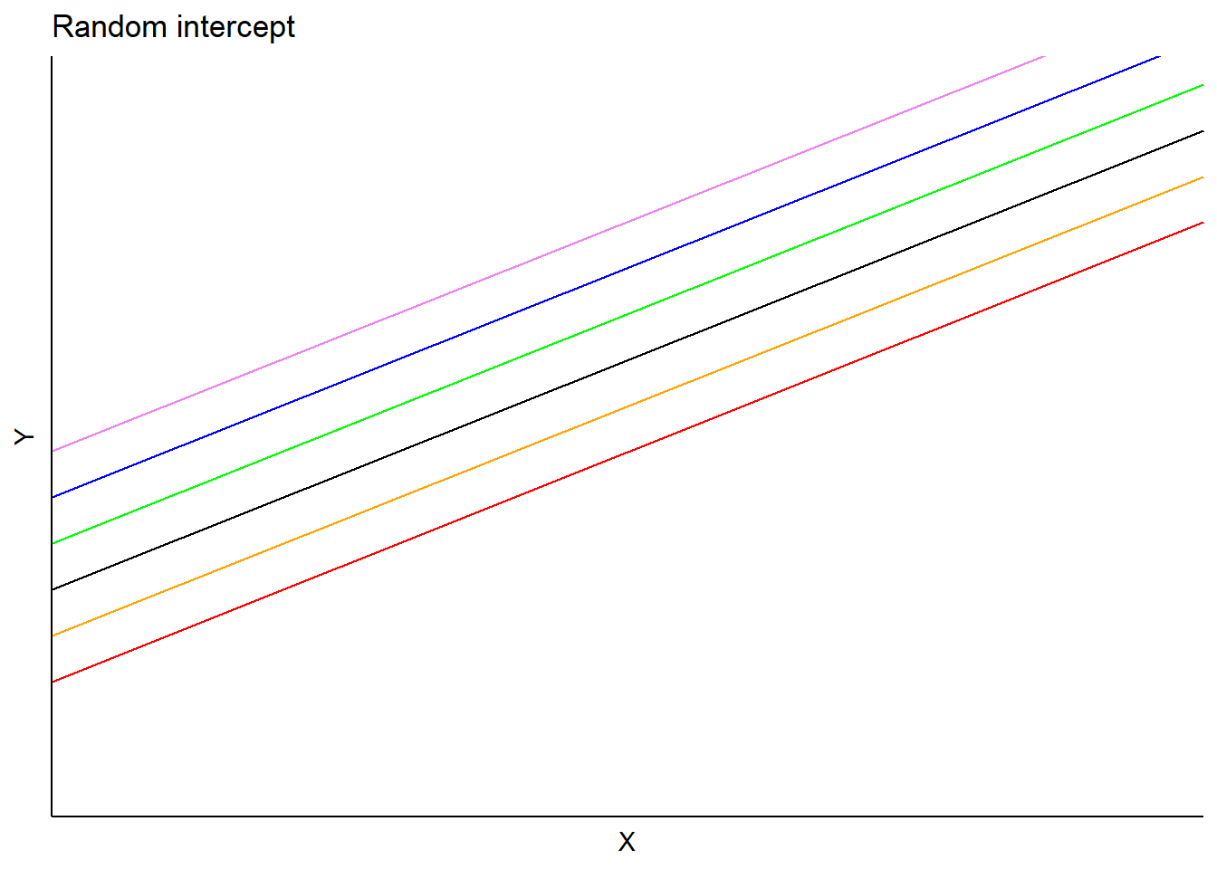
For example, consider a model estimating the heights of trees (response variable) using a tree’s diameter at breast height (predictor variable). A random effect on the intercept can be applied to each stand that a tree resides in. In this model, predictions would vary depending on each subject’s random intercept term, but slopes would be the same:
Similar to applying a random effect term on the intercept, we can instead apply it to the slope term in a regression. This model form would be:
\(Y=\beta_0+(\beta_1+b_i)X+\epsilon\)
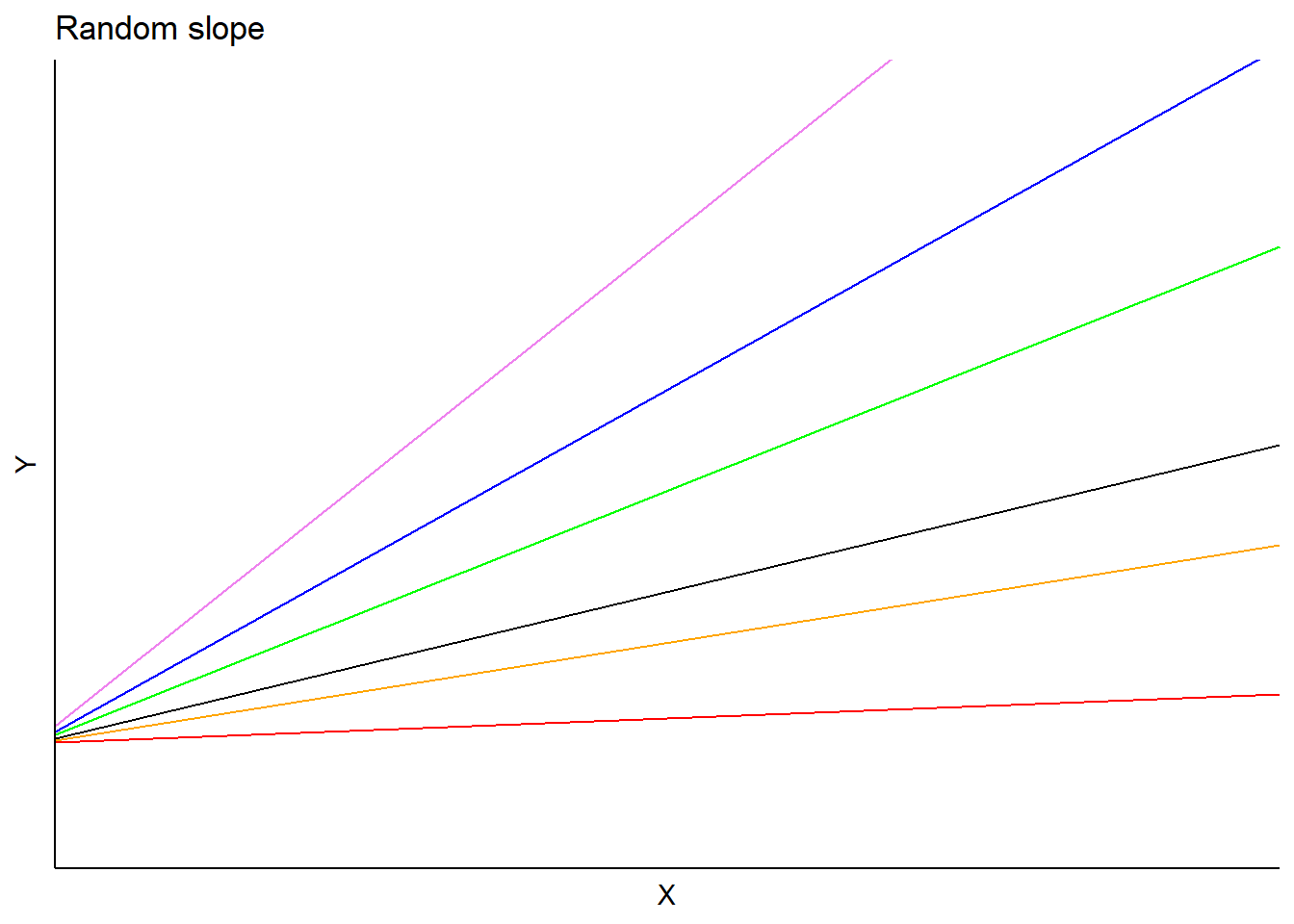
In this model, the \(b_i\) is a random effect for subject \(i\) applied to the slope. Predictions would vary depending on each subject’s random slope term, but the intercept would be the same:
One could also specify a random effect term on both the intercept and slope. In the tree height-diameter example, this would indicate a random effect applied to each stand on the intercept in addition to a random effect for the slope parameter associated with a tree’s diameter in each stand. This model form would be:
\(Y=(\beta_0+a_i)+(\beta_1+b_i)X+\epsilon)\)
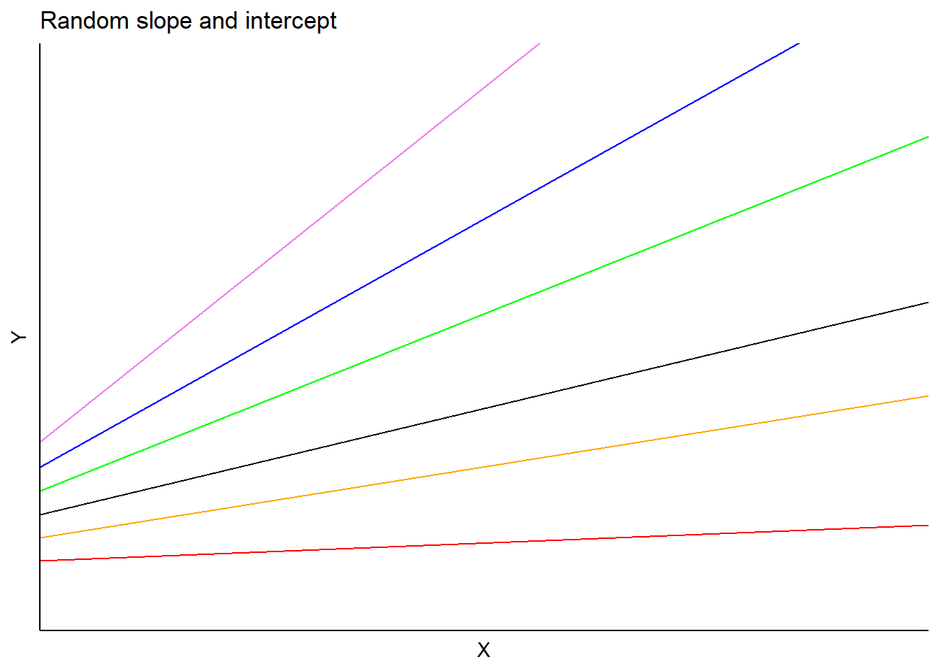
In this model, \(a_i\) and \(b_i\) are random effects for subject \(i\) applied to the intercept and slope, respectively. Predictions would vary depending on each subject’s slope and intercept terms:
One of the most popular applications of mixed models is to consider the nested or hierarchical structure of data. In forestry, a common example is to nest a measurement plot within a forest stand to take into account the hierarchical nature of forest inventory design.
Consider a random effect term applied to the intercept. By nesting subject \(j\) within subject \(i\), this model form would be:
\(Y=(\beta_0+b_i+b_{ij})+\beta_1X+\epsilon\)
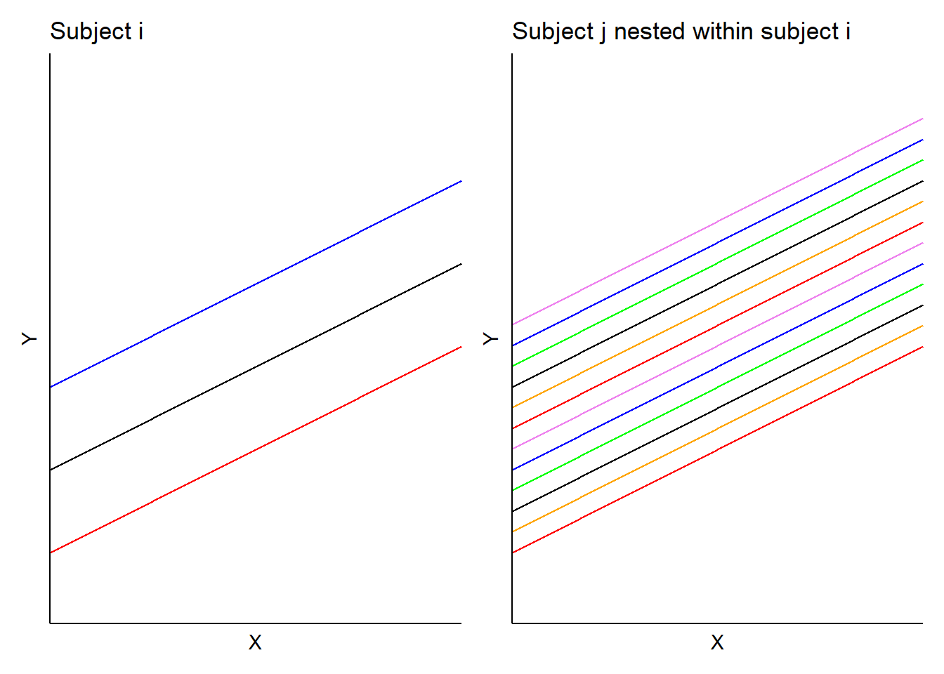
In this model, \(b_i\) is the random effect for subject \(i\) and \(b_{ij}\) is the random effect for subject \(j\) nested in subject \(i\). In the tree height example, we would obtain a set of random effects for each stand and a set of random effects for each plot nested within each stand. Hence, predictions would result in two sets of random effects for each intercept (with identical slopes):
Case study: Predicting tree height with mixed models
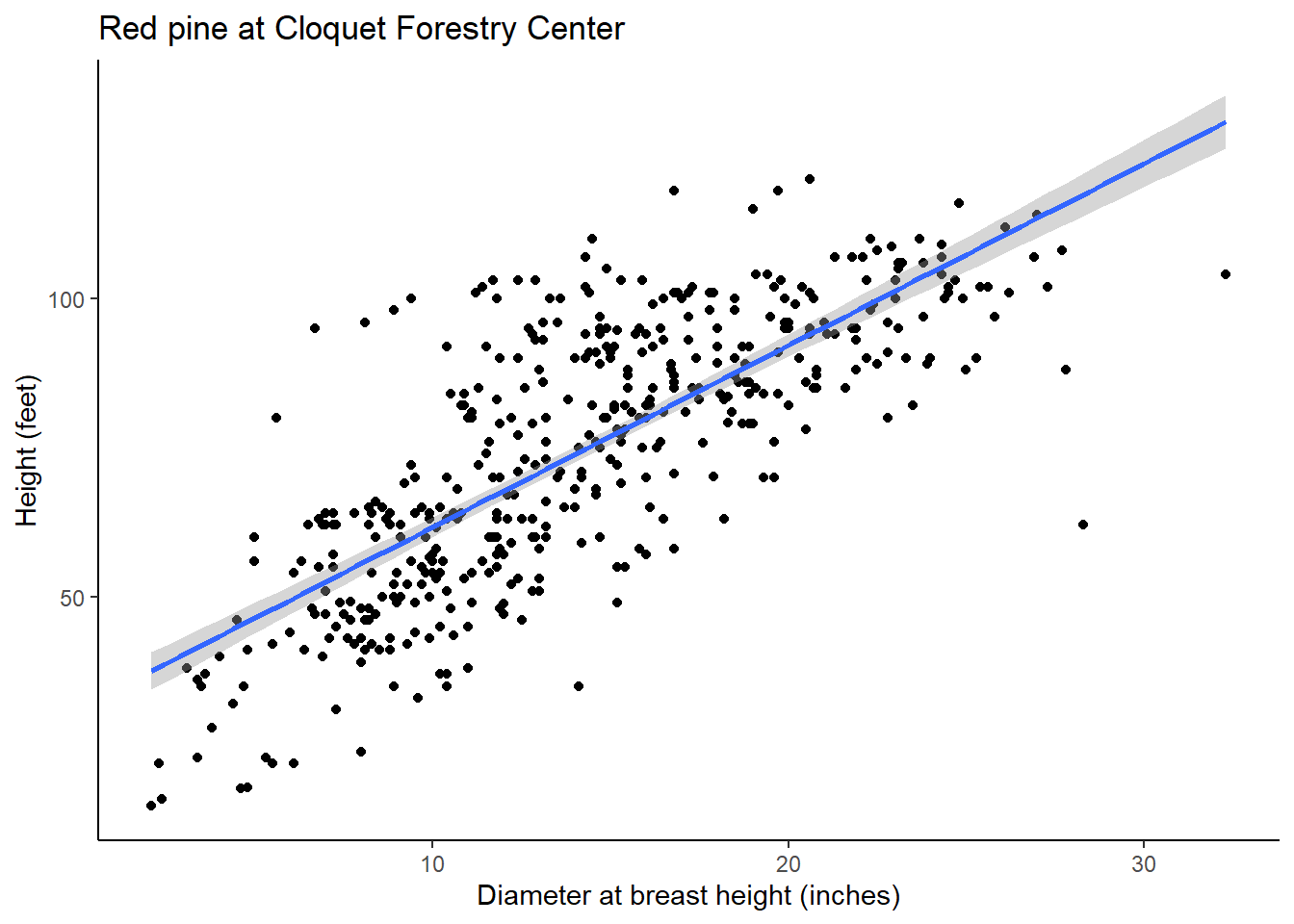
We are interested in predicting a tree’s height (HT) based on its diameter at breast height (DBH). Data are from 450 observations made at the Cloquet Forestry Center in Cloquet, Minnesota in 2014 with DBH measured in inches and HT measured in feet. Data were collected from various cover types and plots across the forest:
| CoverType | PlotNum | TreeNum | DBH | HT |
|---|---|---|---|---|
| Red pine | 5 | 46 | 13.0 | 51 |
| Red pine | 5 | 50 | 8.3 | 54 |
| Red pine | 5 | 54 | 8.2 | 48 |
| Red pine | 5 | 56 | 11.8 | 55 |
| Red pine | 5 | 63 | 9.0 | 54 |
| Red pine | 5 | 71 | 12.5 | 46 |
| Cut | 11 | 47 | 25.3 | 90 |
| Red pine | 13 | 1 | 16.2 | 85 |
| Red pine | 13 | 2 | 18.8 | 86 |
| Red pine | 13 | 7 | 22.2 | 90 |
Ordinary least squares
A ordinary least squares model can be considered as:
\(HT=\beta_0+\beta_1DBH+\epsilon\)
In R, the most common function to perform a simple linear regression like this is lm().
pine.lm <- lm(HT ~ DBH, data = pine)
summary(pine.lm)
##
## Call:
## lm(formula = HT ~ DBH, data = pine)
##
## Residuals:
## Min 1Q Median 3Q Max
## -55.449 -9.250 -0.894 8.878 43.415
##
## Coefficients:
## Estimate Std. Error t value Pr(>|t|)
## (Intercept) 31.1552 1.8357 16.97 <2e-16 ***
## DBH 3.0493 0.1201 25.39 <2e-16 ***
## ---
## Signif. codes: 0 '***' 0.001 '**' 0.01 '*' 0.05 '.' 0.1 ' ' 1
##
## Residual standard error: 14.31 on 448 degrees of freedom
## Multiple R-squared: 0.59, Adjusted R-squared: 0.5891
## F-statistic: 644.7 on 1 and 448 DF, p-value: < 2.2e-16The estimated values of \(\beta_0\) and \(\beta_1\) are 31.1552 and 3.0493, respectively. The R-squared of this regression line is 0.59, indicating a moderate to strong relationship between DBH and HT. This can be observed in the following graph:
Random effects on intercept
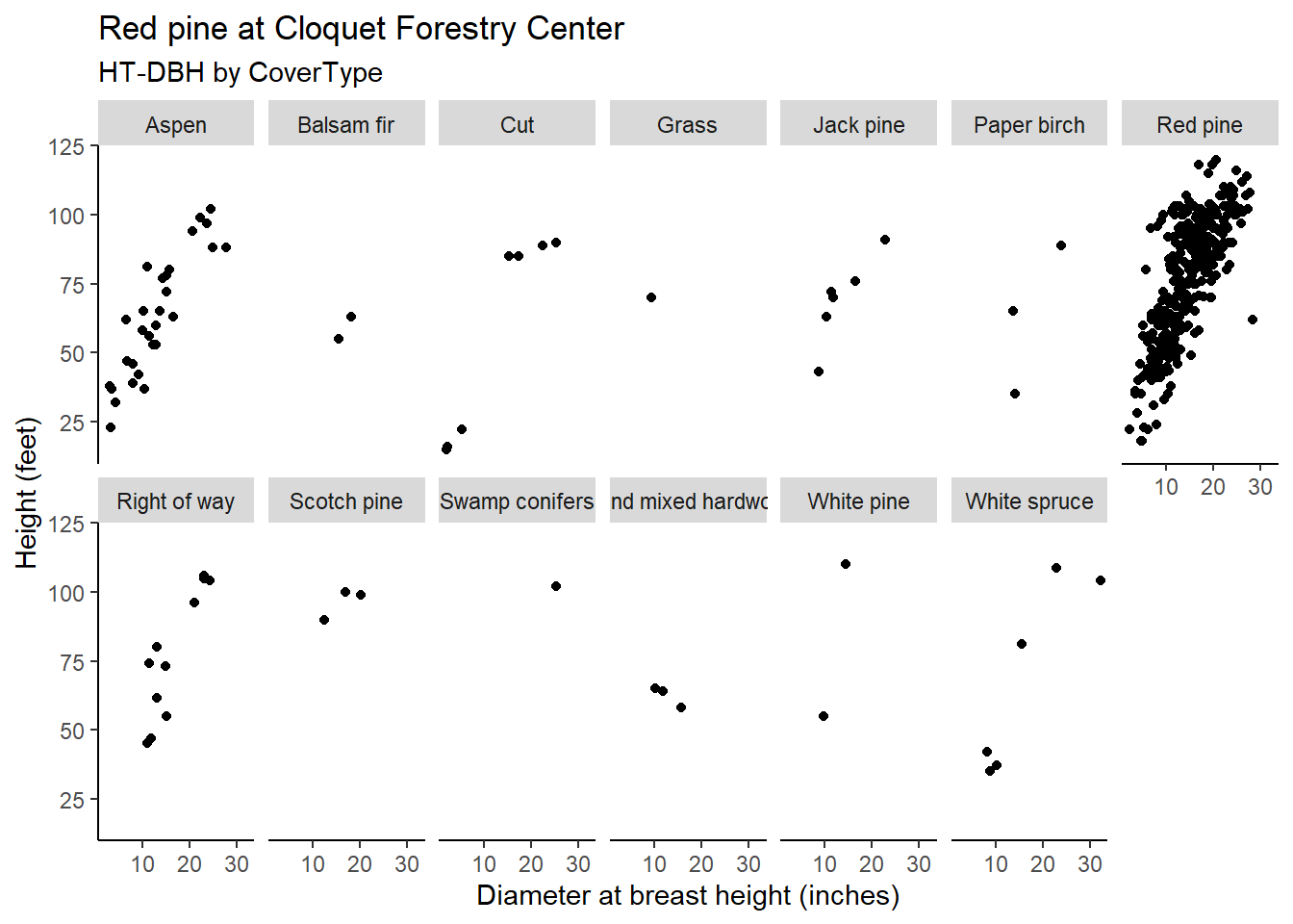
We can expand the simple linear regression to a mixed model by incorporating the forest cover type from where a tree resides as a random effect. In the Cloquet data, the n_distinct() function indicates there are 13 different cover types on the property.
n_distinct(pine$CoverType)## [1] 13We can see that while most of the red pine trees are found in the red pine cover type, the species is also found in the other 12 cover types but are less abundant:
The lme4 package in R can be used to fit linear mixed models for fixed and random effects. We will use it to fit three mixed models that specify random effects on different parameters:
install.packages("lme4")
library(lme4)
The lmer() function is the mixed model equivalent of lm(). To specify the cover type as a random effect on the intercept, we write (1 | CoverType):
pine.lme <- lmer(HT ~ DBH + (1 | CoverType),
             data = pine)
summary(pine.lme)
## Linear mixed model fit by REML ['lmerMod']
## Formula: HT ~ DBH + (1 | CoverType)
## Data: pine
##
## REML criterion at convergence: 3652
##
## Scaled residuals:
## Min 1Q Median 3Q Max
## -4.1165 -0.6923 -0.0591 0.6087 3.0488
##
## Random effects:
## Groups Name Variance Std.Dev.
## CoverType (Intercept) 52.24 7.228
## Residual 191.14 13.825
## Number of obs: 450, groups: CoverType, 13
##
## Fixed effects:
## Estimate Std. Error t value
## (Intercept) 25.8867 3.2321 8.009
## DBH 3.0585 0.1169 26.169
##
## Correlation of Fixed Effects:
## (Intr)
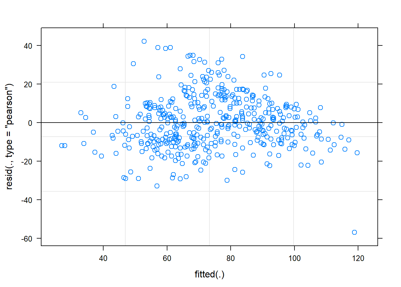
## DBH -0.537We can see from the output that the values for the fixed effects \(\beta_0\) and \(\beta_1\) are 25.8867 and 3.0585, respectively. These values are slightly different from the ordinary least squares. The plot of residuals for the model looks mostly good:
In lme4, the ranef() function extracts the random effect terms. In this model, we can obtain the 13 random effects for each cover type:
ranef(pine.lme)## $CoverType
## (Intercept)
## Aspen -2.4313290
## Balsam fir -6.4569721
## Cut -5.3398733
## Grass 3.2321996
## Jack pine 1.1099090
## Paper birch -7.0258594
## Red pine 6.4705981
## Right of way 0.7999610
## Scotch pine 8.9566777
## Swamp conifers -0.3374007
## Upland mixed hardwoods -0.9416721
## White pine 6.9294464
## White spruce -4.9656851
##
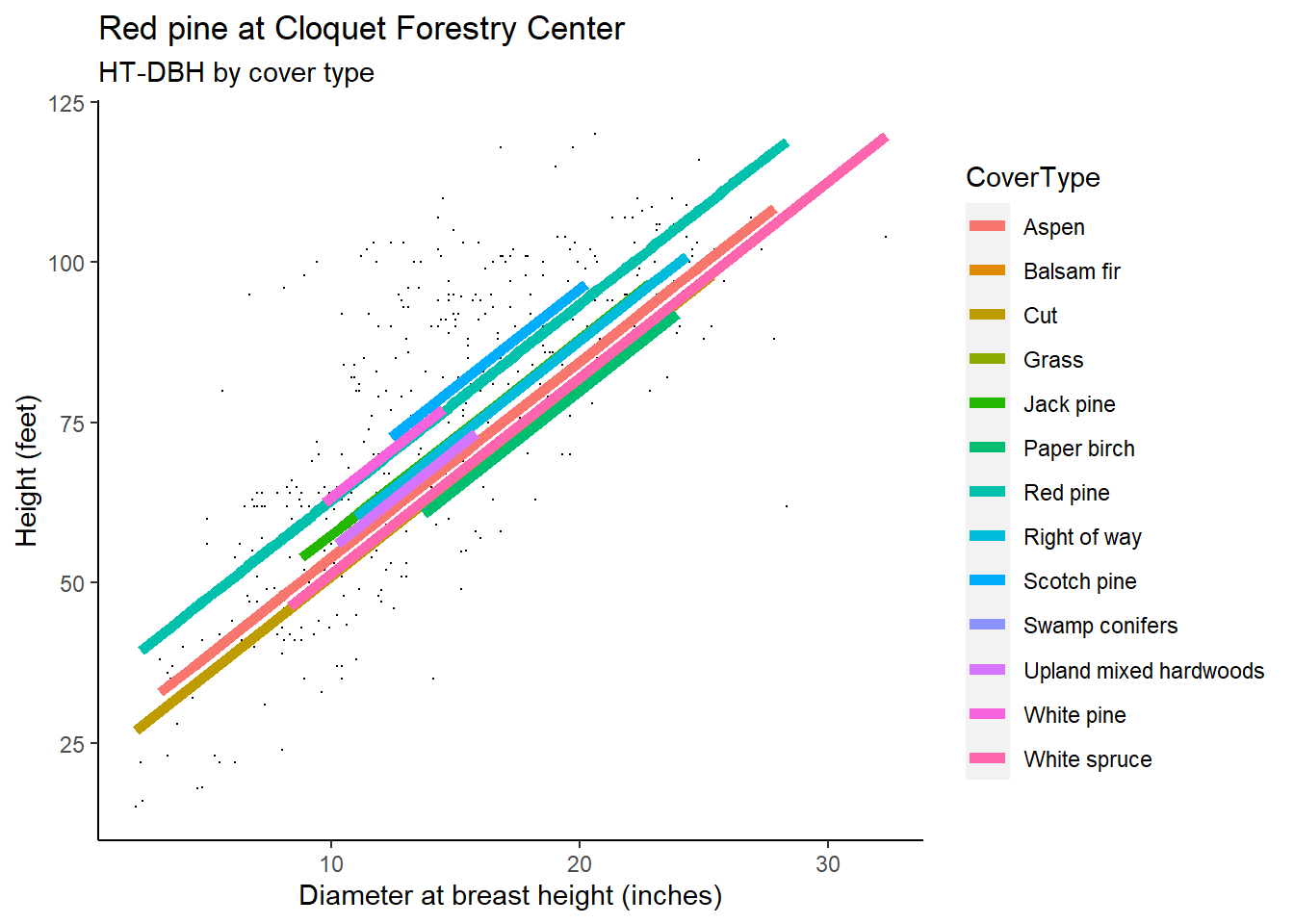
## with conditional variances for "CoverType"As a visual, the HT-DBH models with varying random intercepts shows a different line for each cover type. Note that the lines have the same slope yet different intercepts, as depicted in the random effect term applied to \(\beta_0\). You will notice that some predictions do not extend far through the x-axis, a reflection of the small sample size for red pine trees found in some cover types:
Random effects on slope
An alternative mixed model could be specified by placing a random parameter on the slope term. Adding these random slope terms can introduce a lot of complexity to the model. In the tree height example, we can specify (1 + DBH | CoverType) to place a random effect on the slope term for the DBH term:
pine.lme2 <- lmer(HT ~ 1 + DBH + (1 + DBH | CoverType),
             data = pine)
summary(pine.lme2)
## Linear mixed model fit by REML ['lmerMod']
## Formula: HT ~ 1 + DBH + (1 + DBH | CoverType)
## Data: pine
##
## REML criterion at convergence: 3651.7
##
## Scaled residuals:
## Min 1Q Median 3Q Max
## -4.0915 -0.6998 -0.0553 0.6024 3.0359
##
## Random effects:
## Groups Name Variance Std.Dev. Corr
## CoverType (Intercept) 78.74861 8.8740
## DBH 0.01029 0.1014 -1.00
## Residual 190.92366 13.8175
## Number of obs: 450, groups: CoverType, 13
##
## Fixed effects:
## Estimate Std. Error t value
## (Intercept) 24.9363 3.7333 6.679
## DBH 3.1208 0.1235 25.269
##
## Correlation of Fixed Effects:
## (Intr)
## DBH -0.706
## convergence code: 0
## boundary (singular) fit: see ?isSingularYou can see that the error message boundary (singular) fit: see ?isSingular is shown, indicating that the model is likely overfitted. We may be trying to do too much by specifying the random effects on the slope. Hence, for these data, we might forgo the inclusion of a random slope parameter and instead focus on random effects for the intercept.
Nested random effects on intercept
We can expand the mixed model by incorporating the measurement plot (PlotNum) nested within forest cover type (CoverType) as random effects in the prediction of tree height. In the Cloquet data, there are 124 plots nested within the 13 cover types found in the data.
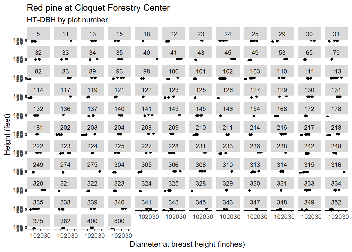
n_distinct(pine$PlotNum)## [1] 124Note the distributions of red pine heights and diameters in each plot. Although difficult to see in each plot, the scatter plots show many plots that contain only a few red pine trees:
To specify nested random effects on the intercept (plot number nested within cover type), we can write (1 | CoverType/PlotNum) in the lmer() function:
pine.lme3 <- lmer(HT ~ DBH + (1 | CoverType/PlotNum),
             data = pine)
summary(pine.lme3)
## Linear mixed model fit by REML ['lmerMod']
## Formula: HT ~ DBH + (1 | CoverType/PlotNum)
## Data: pine
##
## REML criterion at convergence: 3413
##
## Scaled residuals:
## Min 1Q Median 3Q Max
## -3.8376 -0.4860 0.0388 0.5710 3.1585
##
## Random effects:
## Groups Name Variance Std.Dev.
## PlotNum:CoverType (Intercept) 123.63 11.119
## CoverType (Intercept) 19.17 4.378
## Residual 68.73 8.291
## Number of obs: 450, groups: PlotNum:CoverType, 124; CoverType, 13
##
## Fixed effects:
## Estimate Std. Error t value
## (Intercept) 30.5389 2.9080 10.50
## DBH 2.7111 0.1192 22.74
##
## Correlation of Fixed Effects:
## (Intr)
## DBH -0.621In this model, the estimated values of \(\beta_0\) and \(\beta_1\) are 30.5389 and 2.7111, respectively. These values are slightly different from previous model fits. In this model, we can obtain the 13 random effects for each cover type and plot nested within each cover type. A quantile-quantile plot indicates the random effects are generally normally distributed:
## $`PlotNum:CoverType`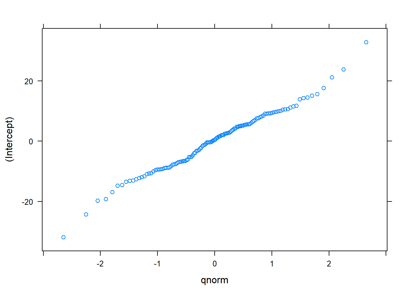
##
## $CoverType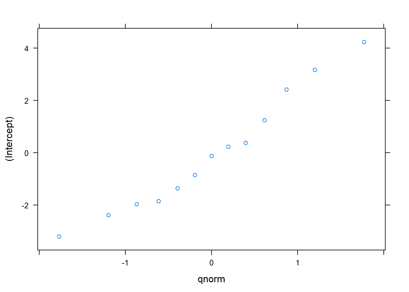
Questions you should ask about mixed models
As you begin to design and implement mixed models in your analysis, a number of questions may come to mind.
Which parameters should be random?
To address this question, you can fit several models with random effects on different parameters. In my experience with forestry data, random effects applied to the intercept are robust and are often the easiest to implement in practice. Random effects applied to slopes encounter more issues with convergence due to their complexity.
After fitting models, you may evaluate them by assessing the quality of each model using metrics such as the Akaike information criterion (AIC) or a likelihood ratio test. We can assess the AIC for the red pine models:
AIC(pine.lm, pine.lme, pine.lme2, pine.lme3)## df AIC
## pine.lm 3 3676.142
## pine.lme 4 3659.952
## pine.lme2 6 3663.716
## pine.lme3 5 3422.994In these models, we would prefer the model with the nested random effects (pine.lme3) because it indicates the lowest AIC compared to the others.
How do you use the equation for subjects not found in the data set?
The mixed modeling framework will work well if you want to predict the height of red pine trees found on these measurement plots. But what about using the equations for subjects not found in the data set?
To do this, one could subsample from the data to get response variables of interest. For example, a person could measure every fourth tree in a measurement plot. Then, random effects can be locally calibrated based on the plot conditions. However, for many forestry variables, such as future volume growth, a subsample of growth measurements are not likely to be available.
Another approach is to set the random effects equal to zero. In this case, one could make fixed effects-only predictions. This approach is similar to the ordinary least squares approach when simply using the coefficients \(\beta_0\) and \(\beta_1\) to make predictions.
Are mixed models needed?
A valid question is to ask whether mixed models are needed or if a more parsimonious model might be preferred. To examine this, try fitting a model with and without random effects. The various model forms can be evaluated with AIC or a likelihood ratio test. In the case of the red pine heights, the lower AIC values for the mixed models indicate that random effects are useful in the predictions
Conclusions
Mixed models are widely used in forestry today. They are effective because forestry data are often spatially and temporally correlated, they can account for hierarchy within data, and they consist of both fixed and random effects. The lme4 package in R is useful for fitting linear mixed models and can include random effects on intercept and slope terms.
Nested random effects are useful because they take into account the hierarchy within forestry data. Multiple models can be fit with different parameters specified as random effects to determine the appropriate random parameters. Using the equations for subjects not found in the data set can be accomplished by using fixed effects parameters only or, with more effort, subsampling from the data to obtain the response variables of interest.
–
Thanks the the University of Minnesota’s Silva Lab for their comments on the presentation of this work.
By Matt Russell. Sign up for my monthly newsletter for in-depth analysis on data and analytics in the forest products industry.