Stratified vs. simple random sampling: fun with forestsamplr
May 22, 2019
sampling forestsamplr forest inventoryTools for estimating population means for stratified and simple random samples
If we know the size of a number of subpopulations that are a part of a larger population, we can use stratified random sampling to come up with a more precise estimate of a population mean. If these subpopulations, or strata, have different mean values and smaller variances relative to the population mean, stratified random sampling is generally preferred over simple random sampling. What this ultimately results in is a narrower confidence interval for an overall population estimate, even when using the same sample size.
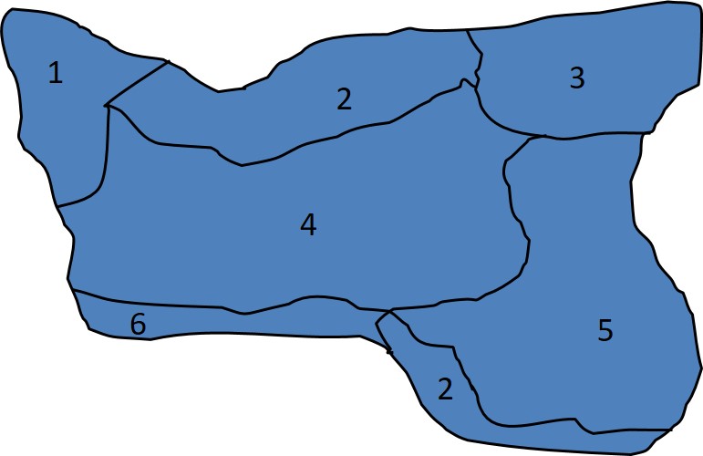
Six example forest stands (or strata).
Stratification is essential in forest inventory planning. Nan Pond and the folks at SilviaTerra recently published the forestsamplr package that can estimate population parameters from a variety of sample designs in a whim (including stratified random samples). The package contains a library of functions for processing natural resource data from a variety of sample designs:
#devtools::install_github("SilviaTerra/forest_sampling")
library(forestsamplr)
When they say a variety of sample designs, they’re not kidding. The functions for simple random sampling and stratified sampling worked well, as outlined below. But there are also functions available for systematic, cluster, Poisson, and two-stage sampling. Functions are even available for 3P sampling!
Tree stocking on the Penobscot Experimental Forest
Data from the Penobscot Experimental Forest were used to compare the differences in population means after sampling trees on permanent sample plots from both five- and ten-year selection harvests. In these harvests, individual trees were harvested at approximate five- and ten-year intervals. The PEF data is a useful dataset for visualizing differences across silvicultural treatments.
This post from March 2019 described two “stands” within each of the five- and ten-year selection harvests. They’re actually defined as experimental units that are a part of the long-term study at the PEF, but for here can be used to investigate the differences between taking stratified and simple random samples. Since the late 1950’s, stands 9 and 16 have been managed under a five-year selection treatment and stands 12 and 20 have been managed under a ten-year selection treatment.
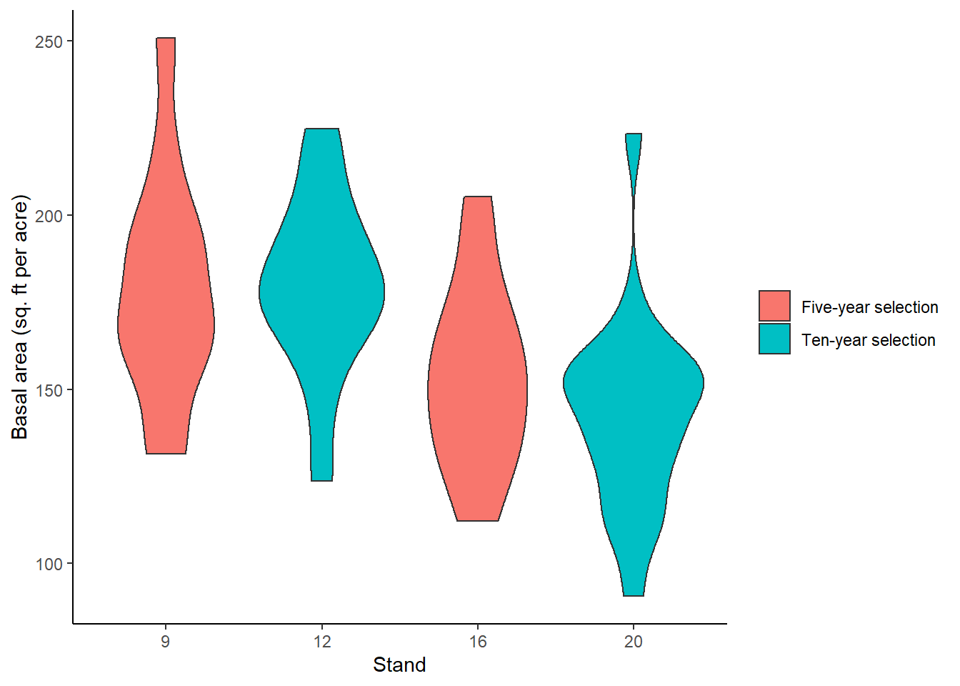
Assume the PEF field crews sampled 68 plots randomly across these four stands, representing a simple random sample. We can store these data in the dataframe plot. The basal area per acre (BAPA, measure in sq. ft per acre) at each plot was the response variable of interest, and we can visualize the differences across the stand using violin plots. Stand 9, a five-year selection treatment, generally had the greatest basal area, followed by the other stands:
| MgmtUnit | Plot | BAPA |
|---|---|---|
| 9 | 11 | 192.3005 |
| 9 | 13 | 199.0091 |
| 9 | 14 | 157.1938 |
| 9 | 21 | 218.3839 |
| 9 | 22 | 131.5173 |
| 9 | 23 | 161.6629 |
Simple random sampling (SRS)
Assuming we measured a SRS with the 68 plots, the population mean of basal area can be calculated using the summarize_all_srs() function in forestsamplr, and a 95% confidence interval is provided in the output:
srs95<-summarize_all_srs(plot,attribute="BAPA")
srs95
## mean variance standardError upperLimitCI lowerLimitCI
## 1 160.4508 999.3899 3.833655 168.1028 152.7988The desired confidence interval can be changed by adding the desiredConfidence statement. As an example, we can output the 66th percent confidence interval for the SRS:
srs66<-summarize_all_srs(plot,attribute="BAPA",desiredConfidence = 0.66)
srs66
## mean variance standardError upperLimitCI lowerLimitCI
## 1 160.4508 999.3899 3.833655 164.135 156.7666There is nothing much surprising about the SRS estimates. A few properties we assume about the SRS are that: (1) we assume the plots were sampled randomly across the four stands, (2) we generally disregard the variability in BAPA within each stand, and (3) we don’t take into account the total area (in acres) of each stand.
Stratified random sampling
The objective of stratification is to minimize variances within a stratum, resulting in a narrower confidence interval with the same size sample. Two additional advantages of conducting a stratified sample are that they (1) provide an estimate of the mean or total for each stratum and (2) provide better spatial coverage of an area. The art of stratification is magical because each within-strata variance is lower than entire population variance. In the case of the four stands at the PEF, the variability of BAPA can be captured within each stand to obtain a more precise estimate of the mean compared to the SRS.
When stratifying, we need to know the area of each of the stands (in our case, acres), which we can create in the stratumTab dataframe:
stratumTab <- data.frame(stratum = c(9,12,16,20), acres = c(27.2,31.3,16.3,21.2))The population mean of BAPA can be calculated using the summarize_stratified() function in forestsamplr, which requires the stratumTab argument that contains the area of each stand. Output is provided for each stand ($stratumSummaries), and then for the entire area ($totalSummary):
strat95<-summarize_stratified(plot,attribute="BAPA",  stratumTab)
strat95
## $stratumSummaries
## stratum stratMean stratVarMean stratSE stratPlots stratAcres
## 1 9 178.8403 81.96929 9.053689 13 27.2
## 2 12 179.7088 48.13725 6.938101 14 31.3
## 3 16 153.5184 34.33973 5.860011 20 16.3
## 4 20 142.8306 36.41038 6.034101 21 21.2
##
## $totalSummary
## popMean popSE popCIhalf ciPct
## 1 166.8719 3.803036 7.597437 4.552857Adding the desiredConfidence statement provides the 66th percent confidence interval for the stratified sample and a useful comparison to SRS:
strat66<-summarize_stratified(plot,attribute="BAPA", stratumTab, desiredConfidence = 0.66)
strat66
## $stratumSummaries
## stratum stratMean stratVarMean stratSE stratPlots stratAcres
## 1 9 178.8403 81.96929 9.053689 13 27.2
## 2 12 179.7088 48.13725 6.938101 14 31.3
## 3 16 153.5184 34.33973 5.860011 20 16.3
## 4 20 142.8306 36.41038 6.034101 21 21.2
##
## $totalSummary
## popMean popSE popCIhalf ciPct
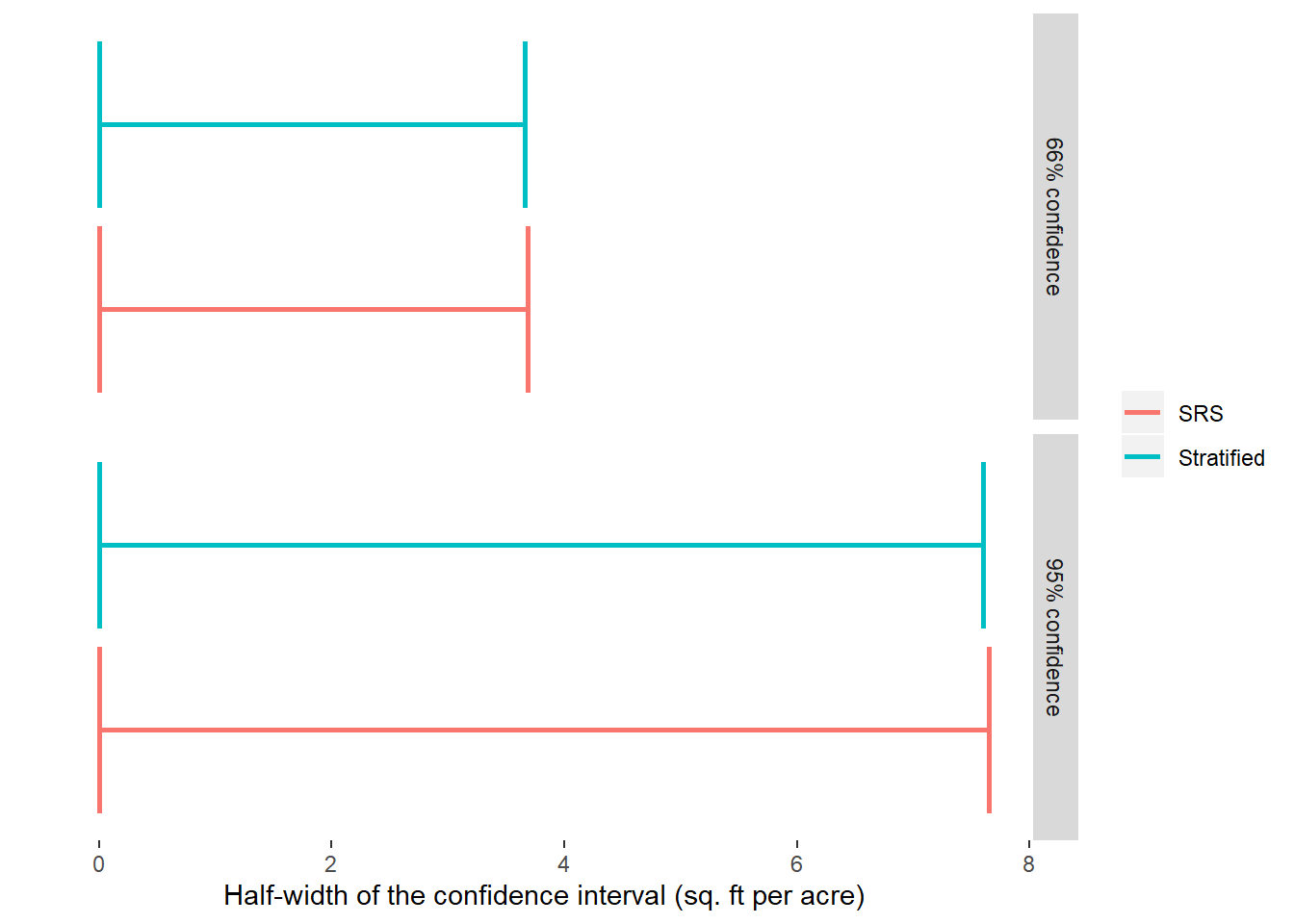
## 1 166.8719 3.803036 3.656005 2.190906The population mean for the stratified sample is slightly larger than for the SRS (166.87 vs. 160.45 sq. ft per acre). The standard error is reduced from 3.83 to 3.80 sq. ft per acre when stratifying. We can see the differences (ever so slightly) in the smaller half-width for the confidence intervals for the stratified sample:
Allocating field plots to stratum
In the sample of field plots at the PEF, it turns out they were laid out in a generally systematic fashion across each stand, ranging from 13 plots in stand 9 to 21 plots in stand 20. Knowing what we now know about the variability within each strata, we could allocate the number of field plots to each stand in a few different ways.
Described in Burkhart et al.’s Forest Measurements, there are two common ways to allocate field plots in a stratified random sample: through proportional or optimal allocation.
Proportional allocation
Say we were interested in taking 150 new field plots across the four stands to estimate BAPA. Proportional allocation would distribute the 150 field plots according to their total area. That is, take more field plots in larger area stands. The propall function allocates the total number of desired plots to each of the stratum. We can apply the function to the stratumTab dataframe:
propall<-function(acres.stratum,total.acres,total.plots){
  num.plots = round((acres.stratum/total.acres)*total.plots)
  return(num.plots)}

stratumTab$n_proportional<-propall(acres.stratum=stratumTab$acres,total.acres=sum(stratumTab$acres),total.plots=150)
Optimal allocation
The optimal allocation method would distibute the 150 field plots to each stratum that provides the smallest amount of variability possible. In addition to the total area, also required in this calculation is the standard deviation of BAPA within each stratum. The total number of plots to sample in each stand would be represented by the stratum area multiplied by the standard deviation of BAPA. The optall function allocates the total number of desired plots to each of the stratum, and we can apply it to the stratumTab dataframe:
optall<-function(area_sd,sum.area_sd,total.plots){
  num.plots = round((area_sd/sum.area_sd)*total.plots)
  return(num.plots)}

stratumTab$n_optimal<-optall(area_sd=stratumTab$area_sd,sum.area_sd=sum(stratumTab$area_sd),total.plots=150)
We can see the differences between optimal and proportional allocation. The largest differences in how the plots are distibuted occur between stand 9 (the stand with the greatest variability in BAPA) and stand 12 (the stand with the lowest variability in BAPA). The optimal allocation strategy indicates sampling seven more plots in stand 9 compared to the proportional allocation method due to the large standard deviation of BAPA. The optimal strategy indicates sampling four fewer plots in stand 12 compared to the proportional allocation method, even though it’s the stand with the largest area.
| stratum | acres | sd_BAPA | area_sd | n_proportional | n_optimal |
|---|---|---|---|---|---|
| 9 | 27.2 | 32.64354 | 887.9043 | 42 | 49 |
| 12 | 31.3 | 25.96000 | 812.5479 | 49 | 45 |
| 16 | 16.3 | 26.20676 | 427.1703 | 25 | 24 |
| 20 | 21.2 | 27.65173 | 586.2166 | 33 | 32 |
The forestsamplr package can easily summarize data from stratified samples and many more designs. Check it out!
By Matt Russell. Leave a comment below or email Matt with any questions or comments.