library(tidyverse)
library(tidymodels)
library(gsheet)
Many people that work with data in R have found the benefits of using the tidyverse suite of packages for cleaning and wrangling data sets. The tidyverse package is a “megapackage” that imports, reshapes, and visualizes data in a consistent manner, among other tasks.
Although cleaning data often consumes the majority of a data scientists time at work, sooner or later something needs to be done with those data. Oftentimes this involves using it to make predictions on new observations, i.e., modeling with regression techniques or machine learning.
The tidymodels package is the tidyverse’s answer to modeling with tidy data. The tidymodels package is a collection of packages that work together to model data in a consistent manner. The package includes functions for preprocessing data, fitting models, and evaluating model performance.
This post will provide a tutorial for using the tidymodels package, along with some important preliminary steps that filter and visualize the data. The goal is to fit a series of models that determine the aboveground biomass of trees using tree diameter as a predictor variable.
Tree biomass data
First, we’ll load in some R packages to use:
Then, we’ll read in the data found in a Google Sheet using the gsheet2tbl() function from the gsheet package. The data contains tree measurements from the US State of Georgia. I’ve gathered data from the Legacy Tree Database, an online repository of individual tree measurements such as volume, weight, and wood density. I queried the database to provide all tree measurements from the US State of Georgia.
The species dataset named spp contains the species code and name for each tree species that we’re interested in. We’ll merge them together to create a new dataset named tree2:
# Read in the data
tree_in <- gsheet2tbl("https://docs.google.com/spreadsheets/d/1HbczWJRzqxSo-mulXkL9PMMV5u45aoWkc8jD_hfSVpI/edit?usp=sharing")

# Make a species file
spp <- tibble (
  SPCD = c(131, 110, 111, 121, 132, 611, 129),
  Species = c("Loblolly pine", "Shortleaf pine", "Slash pine",
              "Longleaf pine", "Virginia pine", "Sweetgum", "Eastern white pine")
)

# Merge tree and species file
tree2 <- inner_join(tree_in, spp)
Before we begin modeling with the data, we’ll want to filter it to remove any missing values in the tree diameter (ST_OB_D_BH; measured in inches) and aboveground dry weight variables (AG_DW; measured in pounds). We’ll also summarize the data to get a sense of the number of trees and the mean, max, and min values for tree diameter and aboveground dry weight.
After the query, there are 608 observations from our seven species that contain a value for ST_OB_D_BH and AG_DW.
# Filter the data
tree <- tree2 |>
  filter(!is.na(ST_OB_D_BH),
         !is.na(AG_DW))

# Summarize the tree data
tree  |>
  group_by(Species) |>
  summarize(`Num trees` = n(),
            `Mean DBH` = round(mean(ST_OB_D_BH, na.rm=T), 1),
            `Max DBH` = max(ST_OB_D_BH, na.rm=T),
            `Min DBH` = min(ST_OB_D_BH, na.rm=T),
            `Mean weight`= round(mean(AG_DW, na.rm=T), 1),
            `Max weight` = max(AG_DW, na.rm=T),
            `Min weight` = min(AG_DW, na.rm=T))|>
  arrange(desc(`Num trees`))
# A tibble: 7 × 8
Species `Num trees` `Mean DBH` `Max DBH` `Min DBH` `Mean weight` `Max weight`
<chr> <int> <dbl> <dbl> <dbl> <dbl> <dbl>
1 Lobloll… 186 3.1 8.5 0.7 37.1 423.
2 Shortle… 100 3 4.9 1.1 26.3 78.5
3 Longlea… 80 3 4.9 1.2 36.5 119.
4 Slash p… 80 3 4.9 1.2 30.6 106.
5 Virgini… 80 3 4.9 1 37.7 128.
6 Sweetgum 42 1.8 3.3 1 7.8 26.5
7 Eastern… 40 3 4.9 1 27.5 67.7
# ℹ 1 more variable: `Min weight` <dbl>Let’s also visualize the data to understand the relationship between tree diameter and aboveground dry weight:
ggplot(tree, aes(ST_OB_D_BH, AG_DW, col = Species)) +
  geom_point() +
  labs(x = "Diameter at breast height (inches)",
       y = "Aboveground dry weight (pounds)") +
  theme(panel.background = element_rect(fill = "NA"),
        axis.line = element_line(color = "black"))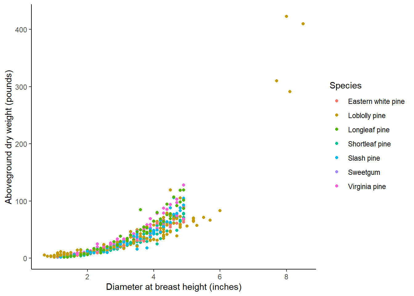
The data contain relatively small trees, with DBH ranging values from 0.7 to 8.5 inches. There are at least 40 observations for seven primary species common to Georgia. These are mostly different kinds of pine trees in addition to one hardwood tree (sweetgum):
Models of aboveground tree biomass
To start our modeling analysis, we can fit a model predicting aboveground dry weight using tree diameter. From above, we can see a clear nonlinear trend in the data, indicating that a nonlinear model is best.
We can fit a nonlinear model using nls() to all observations in the data set. We’ll specify an exponential model that predicts AG_DW as a function of tree diameter. The model has two parameters, b0 and b1, that we’ll estimate. For most nonlinear model fitting functions in R, we’ll need to suggest starting values for the parameters, which we’ll do in the start_vals list. The mod.biomass object fits the model:
bio_pred <- as.formula(AG_DW ~ exp(b0 + b1*log(ST_OB_D_BH)))

start_vals <- list(b0 = -0.02, b1 = 2.5)

mod.biomass <- nls(bio_pred,
             start = start_vals,
             data = tree)
summary(mod.biomass)
Formula: AG_DW ~ exp(b0 + b1 * log(ST_OB_D_BH))

Parameters:
   Estimate Std. Error t value Pr(>|t|)
b0  0.05424    0.05487   0.989    0.323
b1  2.75684    0.03202  86.097   <2e-16 ***
---
Signif. codes:  0 '***' 0.001 '**' 0.01 '*' 0.05 '.' 0.1 ' ' 1

Residual standard error: 12.04 on 606 degrees of freedom

Number of iterations to convergence: 6
Achieved convergence tolerance: 1.519e-06
Here we can see values of 0.05424 and 2.75684 for the b0 and b1 parameters, respectively.
Chapter 24 in the popular book R for Data Science discusses making a grid of data to investigate model predictions. In this step, I’ll use the data_grid() function to generate a grid of data points. Then, I’ll use the add_predictions() function to add the model predictions from tree_mod to complete our data grid. These functions are from the modelr package.
The model appears to perform well:
library(modelr)

grid <- tree |>
  data_grid(ST_OB_D_BH = seq_range(ST_OB_D_BH, 20)) |>
  add_predictions(mod.biomass, "AG_DW")

ggplot(tree, aes(ST_OB_D_BH, AG_DW)) +
  geom_point() +
  geom_line(data = grid, color = "red", linewidth = 1) +
    labs(x = "Diameter at breast height (inches)",
       y = "Aboveground dry weight (pounds)")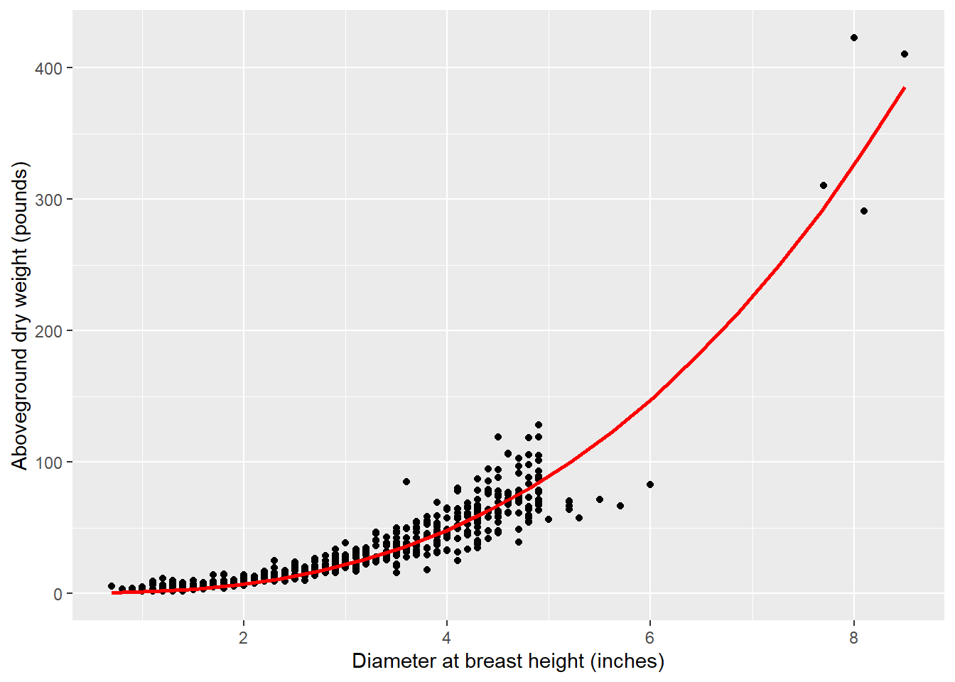
But this model predicts to all of the observations in the tree dataset, and in forestry we like to implement species-specific models. A data analyst’s best friend in the tidyverse is the group_by statement. We can fit the same model as we did earlier, but this time I’ll specify it for each of the seven species using group_by. The tidy() function available in the broom package provides a set of functions that puts model output into data frames.
Here, we can see that the species have a different set of coefficients and other attributes like p-values:
tree_coef <- tree |>
  group_by(Species) |>
   do(tidy(nls(bio_pred, . ,
              start = start_vals)))
tree_coef
# A tibble: 14 × 6
# Groups: Species [7]
Species term estimate std.error statistic p.value
<chr> <chr> <dbl> <dbl> <dbl> <dbl>
1 Eastern white pine b0 0.620 0.180 3.43 1.45e- 3
2 Eastern white pine b1 2.30 0.127 18.1 2.74e- 20
3 Loblolly pine b0 -0.570 0.125 -4.55 9.73e- 6
4 Loblolly pine b1 3.07 0.0655 46.8 3.60e-104
5 Longleaf pine b0 0.394 0.174 2.27 2.61e- 2
6 Longleaf pine b1 2.67 0.119 22.4 9.71e- 36
7 Shortleaf pine b0 0.260 0.144 1.81 7.41e- 2
8 Shortleaf pine b1 2.53 0.100 25.3 9.27e- 45
9 Slash pine b0 -0.170 0.190 -0.891 3.76e- 1
10 Slash pine b1 2.96 0.130 22.7 4.41e- 36
11 Sweetgum b0 0.572 0.0718 7.97 8.82e- 10
12 Sweetgum b1 2.33 0.0758 30.8 1.76e- 29
13 Virginia pine b0 0.804 0.155 5.19 1.60e- 6
14 Virginia pine b1 2.37 0.107 22.2 2.07e- 35A way to visualize the species differences is to plot the intercept and slope coefficients with standard errors. Here we can see that all errors bars do not overlap with zero, indicating they’re good models:
ggplot(tree_coef, aes(estimate, 1)) +
    geom_point() +
    geom_errorbarh(aes(xmin = estimate - (2*std.error),
                       xmax = estimate + (2*std.error),
                       height = 0.25)) +
  scale_y_continuous(limits = c(0,2))+
  facet_grid(term~Species)+
  labs(x = "Coefficient", y = " ")+
  ggtitle("Coefficients for determining aboveground dry weight \n(+/- two standard errors) for seven tree species")+
  theme(axis.text.y = element_blank(),
        axis.ticks.y = element_blank())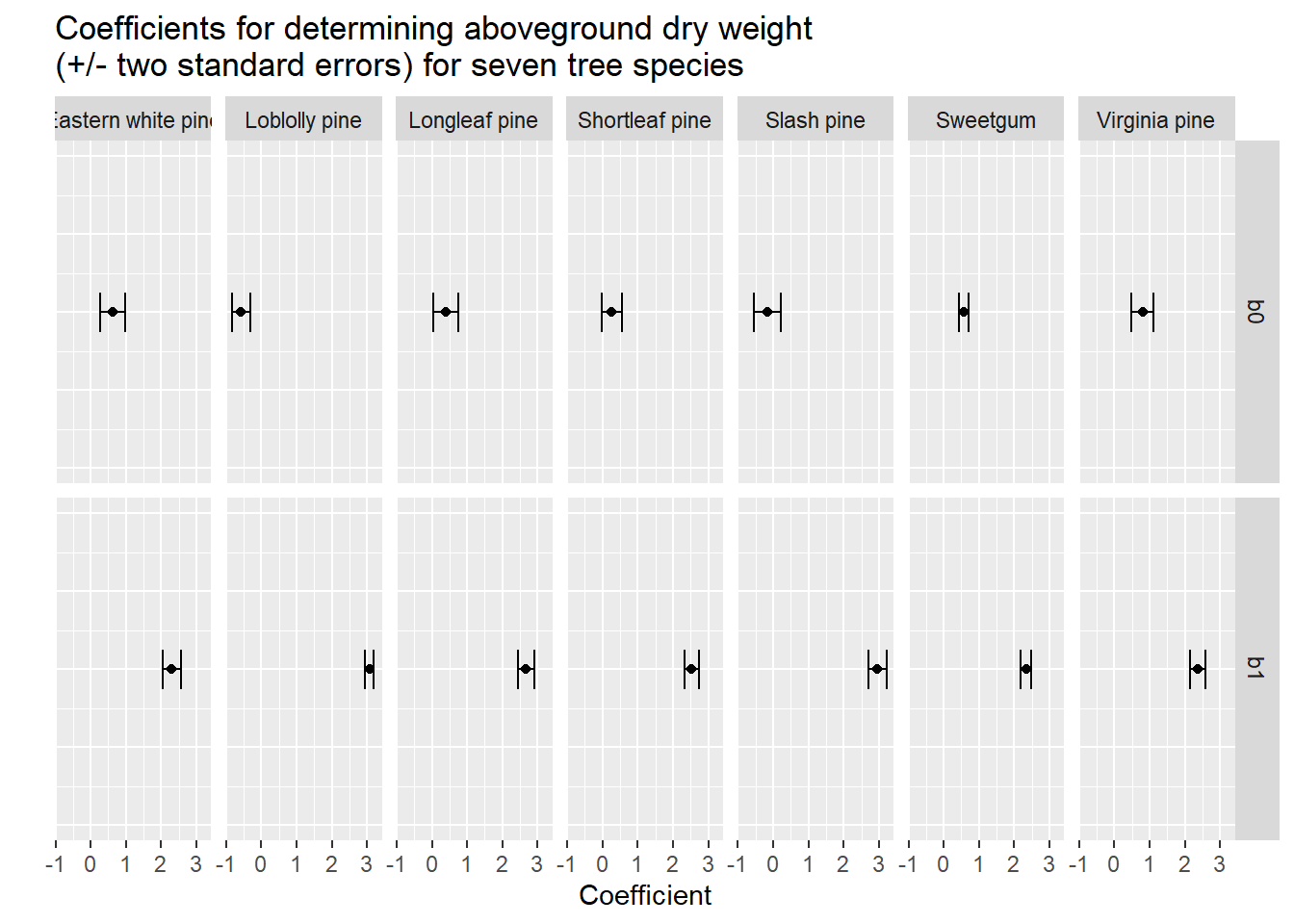
Analysis of model predictions
Aside from coefficients, we might be interested in species-specific predictions from a model. The nest() function creates a list of data frames containing all the nested variables in an object. A nested data frame can be thought of as a “data frame containing many data frames”.
The by_spp object will store this list of data frames for each species so that we can work with them:
by_spp <- tree |>
  group_by(Species) |>
  nest()

species_model <- function(df){
  nls(bio_pred,
      start = start_vals,
      data = tree)
  }

models <- map(by_spp$data, species_model)

by_spp <- by_spp |>
  mutate(model = map(data, species_model))

by_spp
# A tibble: 7 × 3
# Groups: Species [7]
Species data model
<chr> <list> <list>
1 Sweetgum <tibble [42 × 5]> <nls>
2 Loblolly pine <tibble [186 × 5]> <nls>
3 Shortleaf pine <tibble [100 × 5]> <nls>
4 Virginia pine <tibble [80 × 5]> <nls>
5 Eastern white pine <tibble [40 × 5]> <nls>
6 Slash pine <tibble [80 × 5]> <nls>
7 Longleaf pine <tibble [80 × 5]> <nls> Similar to what we did above to the all-species equation, we can map the model predictions to the nested object, adding another variable called preds:
by_spp <- by_spp |>
  mutate(preds = map2(data, model, add_predictions))

by_spp
# A tibble: 7 × 4
# Groups: Species [7]
Species data model preds
<chr> <list> <list> <list>
1 Sweetgum <tibble [42 × 5]> <nls> <tibble [42 × 6]>
2 Loblolly pine <tibble [186 × 5]> <nls> <tibble [186 × 6]>
3 Shortleaf pine <tibble [100 × 5]> <nls> <tibble [100 × 6]>
4 Virginia pine <tibble [80 × 5]> <nls> <tibble [80 × 6]>
5 Eastern white pine <tibble [40 × 5]> <nls> <tibble [40 × 6]>
6 Slash pine <tibble [80 × 5]> <nls> <tibble [80 × 6]>
7 Longleaf pine <tibble [80 × 5]> <nls> <tibble [80 × 6]> Then, we can unnest the model predictions. Unnesting is the opposite of what we’ve done in the previous step. This time we’re taking the nested data frame and turning it into a “regular” data frame.
The model predictions can now be visualized by species to better understand differences in aboveground biomass:
preds <- unnest(by_spp, preds)

ggplot(preds, aes(ST_OB_D_BH, pred)) +
  geom_line(aes(group = Species)) +
  labs(x = "Diameter at breast height (inches)",
       y = "Predicted aboveground\ndry weight (pounds)")+
  facet_wrap(~Species)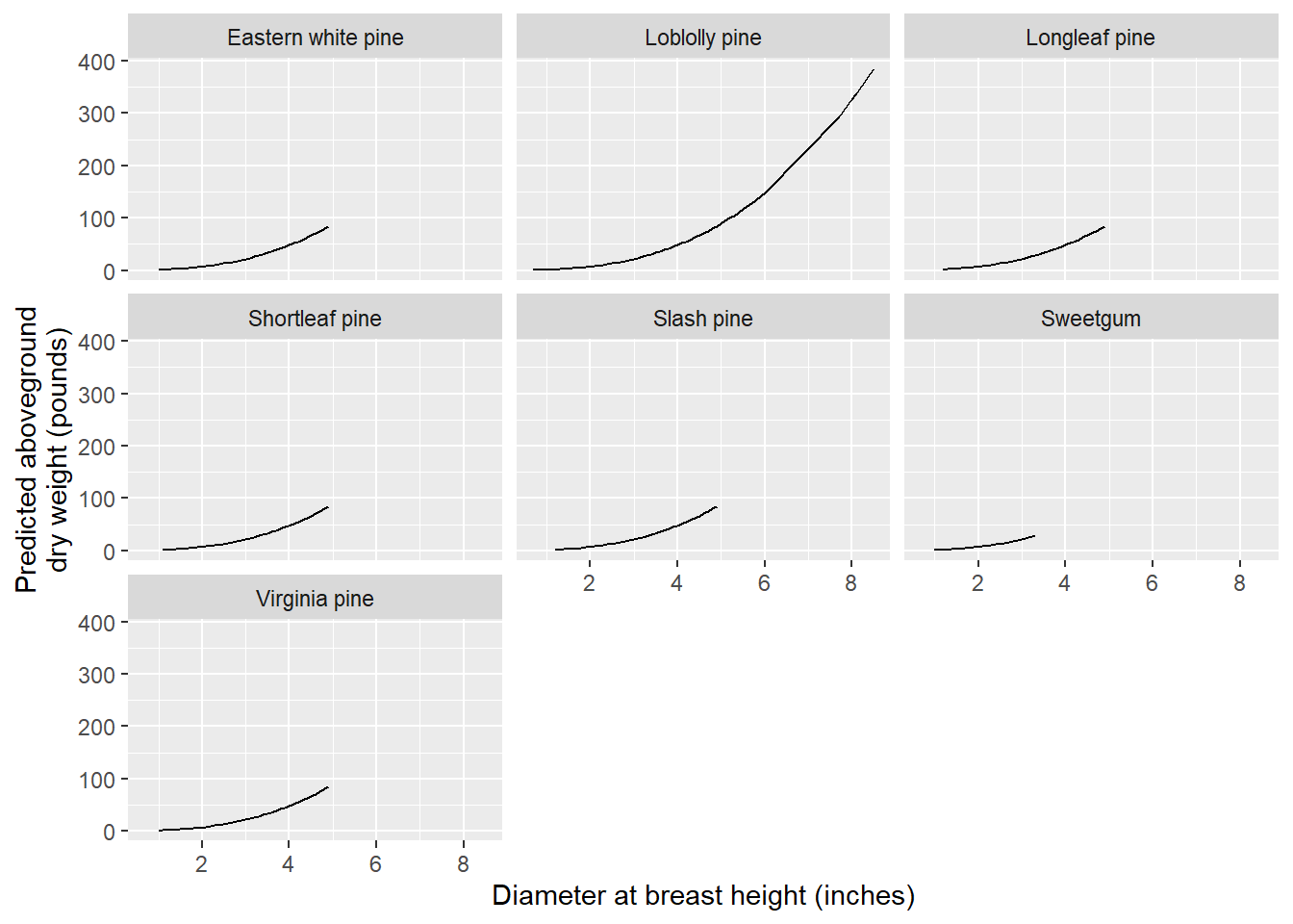
Analysis of model residuals
Any good data analysis involving modeling will also analyze the residuals. Just like we added model predictions with the add_predictions function and nesting/unnesting, we can add residuals with the add_residuals statement. We will go through the same process of nesting, unnesting, and plotting the residuals by species (with a trend line to view any patterns):
by_spp <- by_spp |>
  mutate(resids = map2(data, model, add_residuals))

by_spp
# A tibble: 7 × 5
# Groups: Species [7]
Species data model preds resids
<chr> <list> <list> <list> <list>
1 Sweetgum <tibble [42 × 5]> <nls> <tibble [42 × 6]> <tibble>
2 Loblolly pine <tibble [186 × 5]> <nls> <tibble [186 × 6]> <tibble>
3 Shortleaf pine <tibble [100 × 5]> <nls> <tibble [100 × 6]> <tibble>
4 Virginia pine <tibble [80 × 5]> <nls> <tibble [80 × 6]> <tibble>
5 Eastern white pine <tibble [40 × 5]> <nls> <tibble [40 × 6]> <tibble>
6 Slash pine <tibble [80 × 5]> <nls> <tibble [80 × 6]> <tibble>
7 Longleaf pine <tibble [80 × 5]> <nls> <tibble [80 × 6]> <tibble>resids <- unnest(by_spp, resids)
ggplot(resids, aes(ST_OB_D_BH, resid)) +
geom_point(aes(group = Species), alpha = 1/3) +
geom_smooth(se = F) +
labs(x = "Diameter at breast height (inches)",
y = "Residual")+
geom_abline(intercept = 0, slope = 0, color = "red")+
facet_wrap(~Species)`geom_smooth()` using method = 'loess' and formula = 'y ~ x'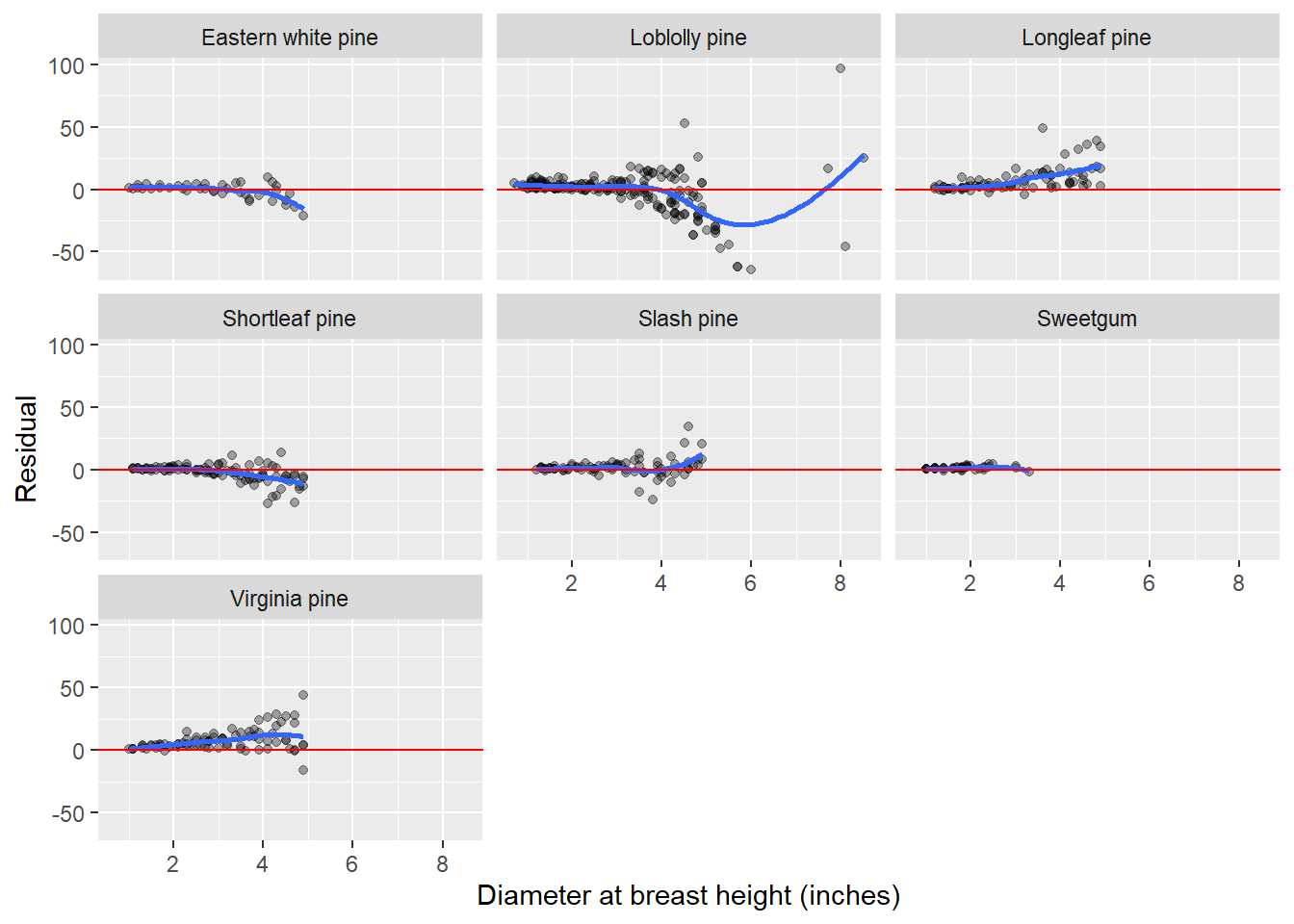
Conclusion
The tidymodels package is an efficient tool for modeling data in R. If you’re familiar with the tidyverse and you also have a need to fit models to data, you will find it useful. It provides a consistent framework for preprocessing data, fitting models, and evaluating model performance.
–
By Matt Russell. For more, subscribe to my monthly email newsletter to stay ahead on data and analytics trends in the forest products industry.