| TREEID | DIA (in) | HT (ft) | Defect, top third | Defect, middle third | Defect, bottom third | Aboveground biomass (lbs) |
|---|---|---|---|---|---|---|
| 1 | 10.5 | 50 | 15 | 10 | 5 | 450.2 |
| 2 | 10.4 | 48 | 10 | 10 | 20 | 448.7 |
| 3 | 8.5 | 41 | 0 | 0 | 0 | 274.8 |
| 4 | 13.0 | 58 | 20 | 5 | 20 | 750.8 |
| 5 | 11.2 | 56 | 10 | 20 | 10 | 522.3 |
| 6 | 12.0 | 60 | 10 | 5 | 5 | 625.1 |
| 7 | 8.8 | 43 | 0 | 0 | 20 | 298.2 |
| 8 | 8.8 | 40 | 10 | 0 | 0 | 302.8 |
| 9 | 10.1 | 54 | 10 | 0 | 0 | 411.4 |
| 10 | 6.9 | 38 | 15 | 10 | 15 | 168.2 |
| 11 | 8.5 | 38 | 20 | 0 | 2 | 274.8 |
| 12 | 10.5 | 52 | 5 | 10 | 12 | 458.9 |
| 13 | 12.1 | 65 | 20 | 10 | 0 | 623.3 |
| 14 | 6.8 | 40 | 5 | 2 | 5 | 162.2 |
| 15 | 7.7 | 42 | 0 | 0 | 0 | 217.2 |
| 16 | 6.8 | 44 | 0 | 0 | 0 | 162.2 |
| 17 | 12.1 | 54 | 0 | 0 | 0 | 623.3 |
| 18 | 12.1 | 58 | 15 | 20 | 5 | 637.2 |
| 19 | 11.1 | 48 | 15 | 0 | 5 | 511.7 |
| 20 | 6.7 | 39 | 20 | 10 | 10 | 156.3 |
Foresters have regularly measured attributes that include tree quality or merchantability as a part of forest inventories. This can include assessments of whether or not the tree meets a sawlog grade, if it shows sweep or another characteristic of poor form, or if it contains defect. Trees are rarely perfect geometric specimens, so incorporating aspects of tree quality can help refine estimates of the tree’s volume.
Increasingly, tree quality is being incorporated into estimates of tree-level biomass and carbon assessments. For example, the amount of cull in a tree is a key parameter used in the National Scale Volume-Biomass Estimators (NSVB), a recently developed set of equations by the USDA Forest Service. The percent defect in different portions of a tree is a component of the American Carbon Registry’s 2.1 methodology for non-Federal forestlands in the US.
If foresters will be measuring tree quality as a part of forest carbon inventories, it’s best to make use of those data and integrate them into estimates of tree volume, biomass, and carbon. This post provides an example for doing this under the ACR methodology.
Aspen biomass data
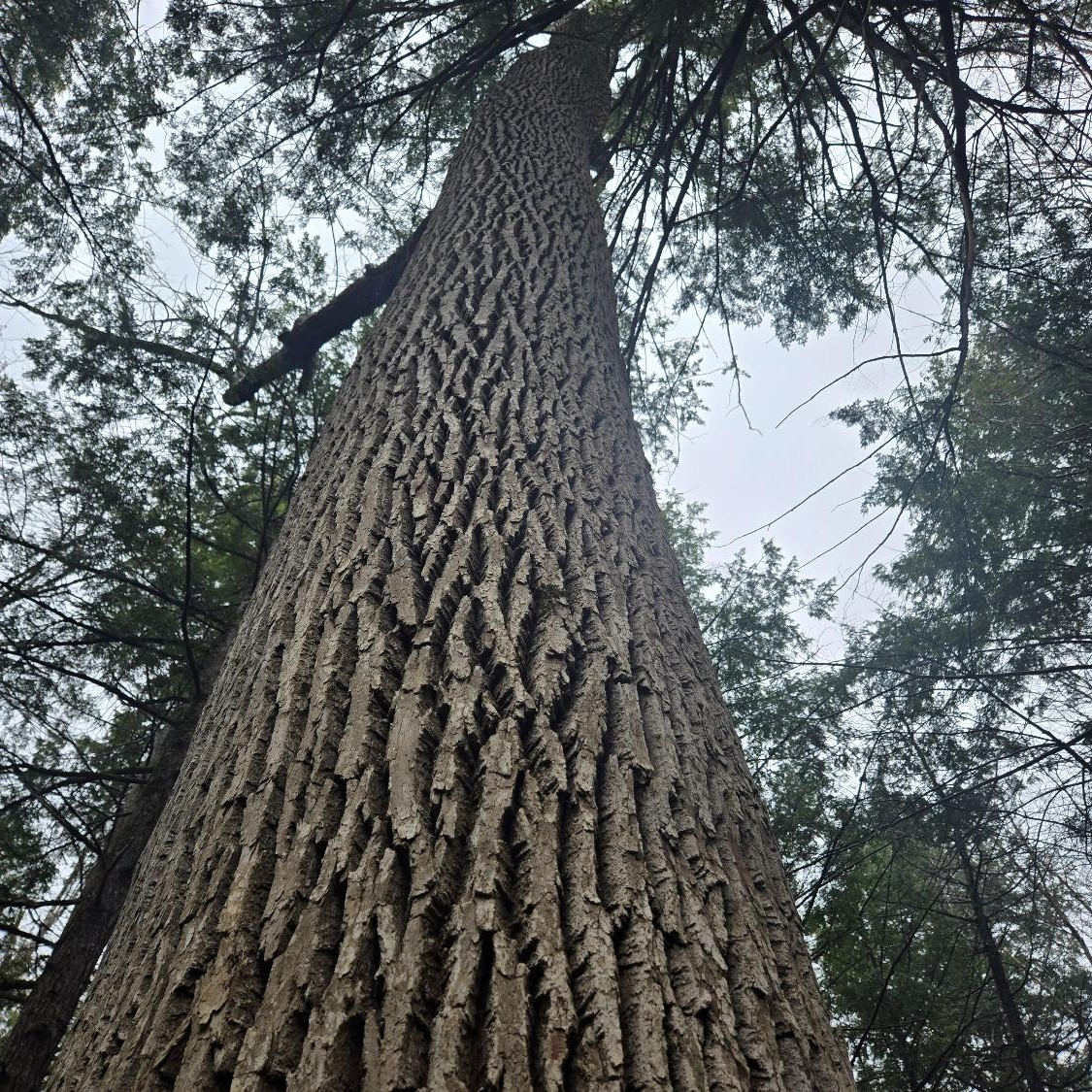
Twenty aspen trees from Minnesota, USA are used as example data. On these trees, diameter at breast height ranged from 6.7 to 13.0 inches. The estimate of aboveground biomass is from the Component Ratio Method (CRM). A set of regional volume equations drive the CRM approach, which are then converted to tree biomass.
There are also field measurements of tree defect in the top, middle, and bottom thirds of the stem. These estimates of defect range from 0 to 20%, depending on the tree and the stem portion. These data are measured to represent the percent missing volume from each third of the tree.
Here are the data collected on the 20 aspen trees and their biomass predictions from the CRM models:
To incorporate tree defect into the estimates of tree biomass, we’ll follow the approach outlined in the ACR’s 2.1 methodology (their Table 5). In this approach, the biomass of each tree can be thought of by dividing the biomass up in thirds (e.g., top, middle, and bottom portions of the stem). This is outlined in the ACR methodology (see their Table 5):
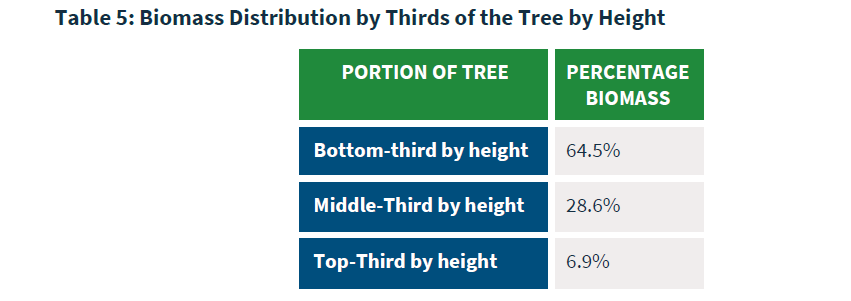
In R, we can reduce the biomass of each tree by accounting for tree defect. First, we’ll multiply the total aboveground biomass by the proportional amount stored within each third of the tree, according to the ACR methodology:
tree <- tree |>
  mutate(biomass_top = AGB * 0.069,
         biomass_mid = AGB * 0.286,
         biomass_bottom = AGB * 0.645)
Second, we’ll multiply by the amount of biomass in each third by the percent of defect noted within that section:
tree <- tree |>
  mutate(top_defect = biomass_top*(defect_pct_top/100),
         mid_defect = biomass_mid*(defect_pct_mid/100),
         bottom_defect = biomass_bottom*(defect_pct_bottom/100))
Lastly, we’ll subtract the amount of defect biomass in each third section by the total “non-defected” portion of tree biomass. Then we’ll add up each section to have a new estimate of total aboveground biomass for each tree, including defect:
tree <- tree |>
mutate(biomass_top_defect = biomass_top - top_defect,
biomass_mid_defect = biomass_mid - mid_defect,
biomass_bottom_defect = biomass_bottom - bottom_defect,
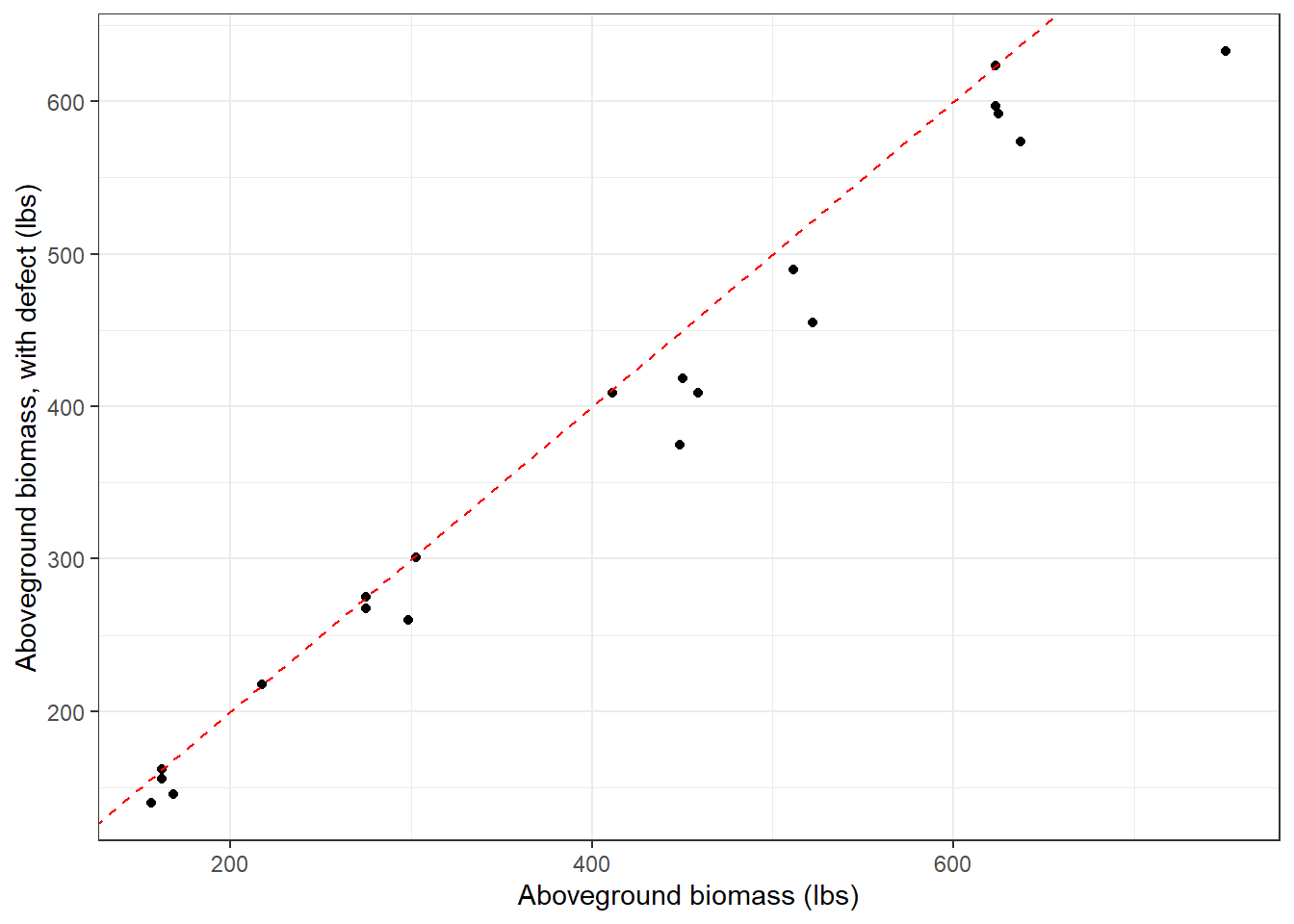
AGB_defect = round(biomass_top_defect + biomass_mid_defect + biomass_bottom_defect, 1))As you can see, incorporating tree defect reduces total aboveground biomass for trees, in this example from 0 to 16.4%:
| TREEID | Aboveground biomass (lbs) | Aboveground biomass, with defect (lbs) | Percent decrease |
|---|---|---|---|
| 1 | 450.2 | 418.1 | 7.1 |
| 2 | 448.7 | 374.9 | 16.4 |
| 3 | 274.8 | 274.8 | 0.0 |
| 4 | 750.8 | 632.8 | 15.7 |
| 5 | 522.3 | 455.1 | 12.9 |
| 6 | 625.1 | 591.7 | 5.3 |
| 7 | 298.2 | 259.7 | 12.9 |
| 8 | 302.8 | 300.7 | 0.7 |
| 9 | 411.4 | 408.6 | 0.7 |
| 10 | 168.2 | 145.4 | 13.6 |
| 11 | 274.8 | 267.5 | 2.7 |
| 12 | 458.9 | 408.7 | 10.9 |
| 13 | 623.3 | 596.9 | 4.2 |
| 14 | 162.2 | 155.5 | 4.1 |
| 15 | 217.2 | 217.2 | 0.0 |
| 16 | 162.2 | 162.2 | 0.0 |
| 17 | 623.3 | 623.3 | 0.0 |
| 18 | 637.2 | 573.6 | 10.0 |
| 19 | 511.7 | 489.9 | 4.3 |
| 20 | 156.3 | 139.6 | 10.7 |
This approach allows one to use detailed field measurements of tree defect to arrive at more refined estimates of tree biomass and carbon. Not incorporating tree defect can lead to overestimates of forest carbon, especially when scaled to the stand or project level.
–
By Matt Russell. Email Matt with any questions or comments.