| State | Parameter | Mean (mtCO2-e/ac) | StdDev (mtCO2-e/ac) |
|---|---|---|---|
| Maine | Live trees | 85.3 | 25.2 |
| Maine | Standing dead trees | 2.8 | 3.0 |
| Maine | Harvested wood products | 0.5734 | 0.3736 |
| Colorado | Live trees | 126.9 | 46.7 |
| Colorado | Standing dead trees | 27.3 | 22.2 |
| Colorado | Harvested wood products | 0 | 0 |
One of the most important attributes when evaluating the extent of stocks in a forest carbon project is the uncertainty. Uncertainty arises from many sources, often including the forest inventory where carbon stocks are estimated. Uncertainty is influenced by how many inventory plots have been collected, how variable the property is, and whether or not stratification was used to reduce variability.
Accurately characterizing uncertainty in a baseline scenario is a critical step in the ACR’s Improved Forest Management (IFM) 2.1 methodology because uncertainty directly affects how many carbon credits a project can ultimately generate.
Uncertainty in the baseline scenario is defined as the weighted average uncertainty across all included carbon pools, with each pool’s uncertainty weighted by its proportional size. When the baseline uncertainty (expressed as a percentage) exceeds the ACR Standard’s ±10% precision threshold, it triggers an uncertainty deduction that reduces the number of issued credits.
The baseline uncertainty calculation (Eq. 12 in the ACR IFM 2.1 methodology) draws on the 90% confidence interval using forest inventory data for live tree and harvested wood products and (optionally) dead wood pools. So, a precise forest inventory filters through the entire uncertainty accounting framework:
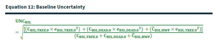
So how sensitive are the components of the baseline uncertainty equation? This post describes a sensitivity analysis of the baseline uncertainty calculation based on example stands from the Forest Inventory and Analysis program.
FIA data
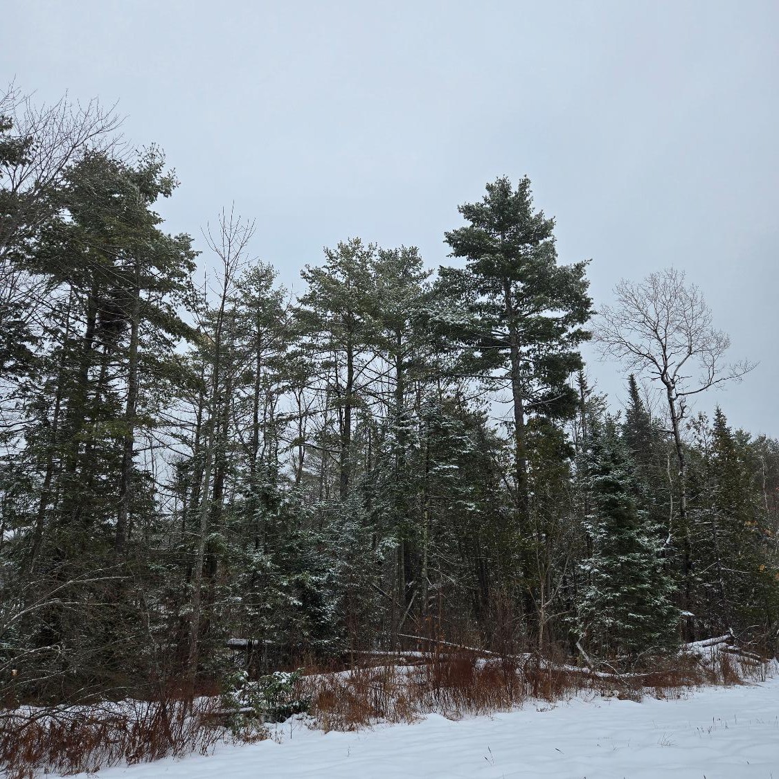
The baseline uncertainty equation requires summary statistics (e.g., mean, standard deviation, and number of plots) of carbon stocks in live trees, dead trees, and harvested wood products. For this purpose, I’ll summarize standing dead trees to represent the dead wood pool. All FIA data measured in the recent inventory were collected from two counties and forest types: spruce-fir forests in Penobscot County, Maine and fir-spruce-mountain hemlock forests in Gunnison County, Colorado. The first represents a forest type that sees active management with little disturbance, while the latter a forest type that sees little management with many recent disturbances (i.e., insect damage to conifer trees in the Rocky Mountain region).
Three key variables were obtained from Forest Inventory and Analysis data using the EVALIDator web application:
- Aboveground and belowground carbon in live trees
- Aboveground and belowground carbon in standing dead trees
- Average annual harvest removals of merchantable bole bark and wood biomass of trees
Forest carbon stocks varied notably between the two regions. In Maine, live trees in spruce-fir forests stored an average of 85.3 mtCO2-e/ac (SD = 25.2), while standing dead trees contributed a modest additional 2.8 mtCO2-e/ac (SD = 3.0), and harvested wood products accounted for 0.57 mtCO2-e/ac (SD = 0.37). In Colorado, forests had considerably higher live tree carbon stocks, averaging 126.9 mtCO2-e/ac (SD = 46.7) along with substantially higher standing dead tree stocks of 27.3 mtCO2-e/ac (SD = 22.2). The FIA data did not record any recent harvests in the Colorado example, hence, harvested wood products carbon was 0.
Sensitivity analysis of uncertainty in carbon pools
To understand which inputs most drive baseline uncertainty, I conducted a one-at-a-time (OAT) sensitivity analysis using FIA plot data. Each of the six key parameters entering Equation 12 (i.e., the per-acre carbon stocks and standard deviations for live trees, standing dead trees, and harvested wood products) was varied independently across a ±50% range of its default value while holding all other parameters at their observed values. The resulting baseline uncertainty (UNCBSL) was recorded at each step.
In Maine, baseline uncertainty using mean and standard deviations was calculated to be 4.3%. The tornado chart below revealed which inputs most impacted uncertainty. Live tree carbon stocks (c_tree_ac) and its standard deviation (sd_tree_ac) dominated the uncertainty output in Maine. Standing dead wood and HWP standard deviation contributed relatively little to overall baseline uncertainty given the smaller stocks in these pools.
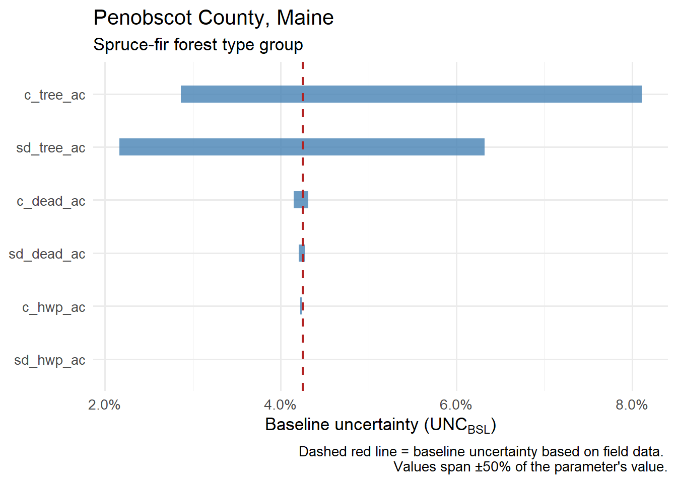
The sensitivity analysis quantifies the influence of each parameter on baseline uncertainty across its ±50% range. Live tree carbon stock (c_tree_ac) produced the largest total swing, with UNCBSL ranging from 2.9% at −50% of its default value to 8.1% at +50%, a total swing of 5.2 percentage points. Even at the greatest swing, UNCBSL falls at 8.1%, within the ACR Standard’s ±10% threshold:
| parameter | UNC_BSL at −50% (%) | UNC_BSL at +50% (%) | Total swing (pp) |
|---|---|---|---|
| c_tree_ac | 2.862 | 8.108 | 5.246 |
| sd_tree_ac | 2.166 | 6.317 | 4.152 |
| c_dead_ac | 4.148 | 4.316 | 0.168 |
| sd_dead_ac | 4.205 | 4.273 | 0.068 |
| c_hwp_ac | 4.223 | 4.239 | 0.016 |
| sd_hwp_ac | 4.231 | 4.231 | 0.000 |
In Colorado, baseline uncertainty was higher at 6.4%. The tornado chart below revealed that standing dead tree carbon stocks had more of an influence on the uncertainty, attributed to the larger dead wood stocks. Still, live tree carbon stocks (c_tree_ac) and its standard deviation (sd_tree_ac) had the greatest influence on uncertainty.
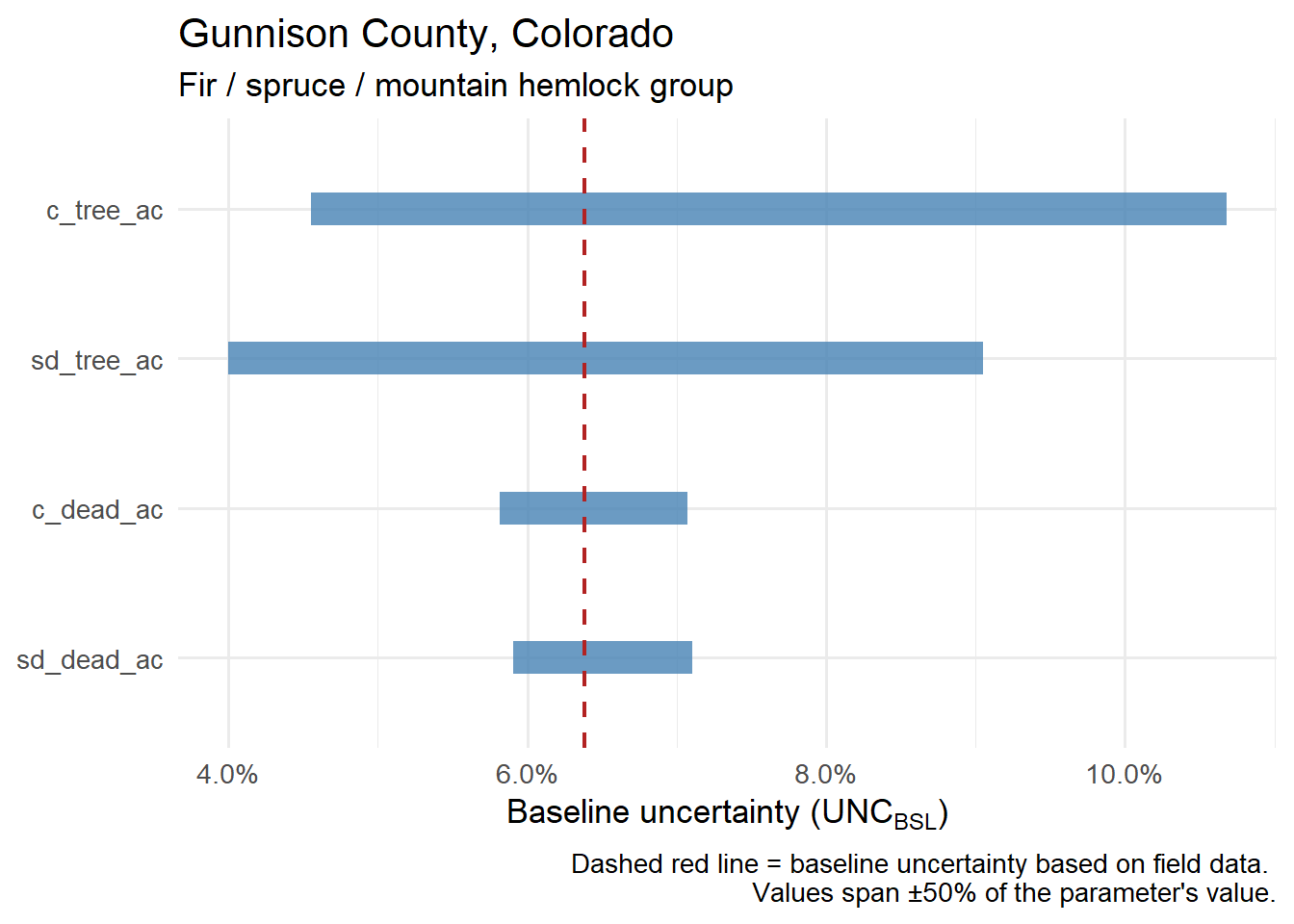
Similar to Maine, live tree carbon stocks produced the largest total swing in the estimate of uncertainty in Colorado’s fir-spruce-mountain hemlock forests, with UNCBSL ranging from 4.5% at −50% of its default value to 10.7% at +50%, a total swing of 6.1 percentage points. This time, at its greatest swing the baseline uncertainty falls outside of ACR Standard’s ±10% threshold, which would trigger an uncertainty deduction:
| parameter | UNC_BSL at −50% (%) | UNC_BSL at +50% (%) | Total swing (pp) |
|---|---|---|---|
| c_tree_ac | 4.551 | 10.683 | 6.132 |
| sd_tree_ac | 4.000 | 9.053 | 5.053 |
| c_dead_ac | 5.816 | 7.072 | 1.256 |
| sd_dead_ac | 5.909 | 7.102 | 1.192 |
This sensitivity analysis illustrates the importance of inventory precision and how sensitive future credit issuance can be to it. Reducing baseline uncertainty should focus on where the carbon is, i.e., in live tree pools in Maine or in live and standing dead pools in Colorado.
These results highlight that the forest inventory serves as the foundation upon which carbon credit generation rests. In particular, the precision of live tree measurements filters through every stage of the uncertainty accounting framework. For landowners and project developers considering an IFM carbon project, don’t underestimate the value of a well-designed forest inventory to start with.
–
By Matt Russell. Subscribe to our monthly email newsletter for data and analytics trends in the forest products industry.